Econ 203 Project - Full Example

Importing the data from an Excel file

Set up your working directory and download this data. After that, install all the packages and use the function read.xlsx() to import the Excel file.

setwd("C:/Users/marce/Desktop/Econ 203 RP")

## If you don't have those packages, start with
## libs <- c("stargazer","ggrepel","ggplot2","ggthemes","extrafont","grid","gridExtra","cowplot","xlsx","dplyr","GGally")
## lapply(libs, install.packages, character.only = TRUE)

libs <- c("stargazer","ggrepel","ggplot2","ggthemes","extrafont","grid","gridExtra","cowplot","xlsx","dplyr","GGally")
lapply(libs, require, character.only = TRUE)

## This is the PISA scores from a bunch of countries (that's my dependent variable). I have also the Government ## spending in education as a fraction of GDP and the Government Efficiency Index.  

PISA<-read.xlsx("dataPISA.xlsx", sheetName = "database", as.data.frame = T, header = T)
View(PISA)

Modifying the dataset

Scale the PISA scores on math applying the natural logarithm function. That transformation on the dependent variable is something that you would do to deal with violations of normality and homoskedasticity assumptions in your model. Also, use the ifelse() function to create dummy variables.

## Ln() of Dependent Variable
PISA$ln_score<-log(PISA$Math.Score.PISA, base=exp(1))

## Creating dummy vaiables
summary(PISA$Continent)

## My baseline is Europe
PISA$Africa<-ifelse(PISA$Continent=="Africa",1,0)
PISA$Asia<-ifelse(PISA$Continent=="Asia",1,0)
PISA$NorthAmerica<-ifelse(PISA$Continent=="North America",1,0)
PISA$Oceania<-ifelse(PISA$Continent=="Oceania",1,0)
PISA$SouthAmerica<-ifelse(PISA$Continent=="South America",1,0)

## New data set with ln() and dummies
View(PISA)

Step 1: Scatterplots

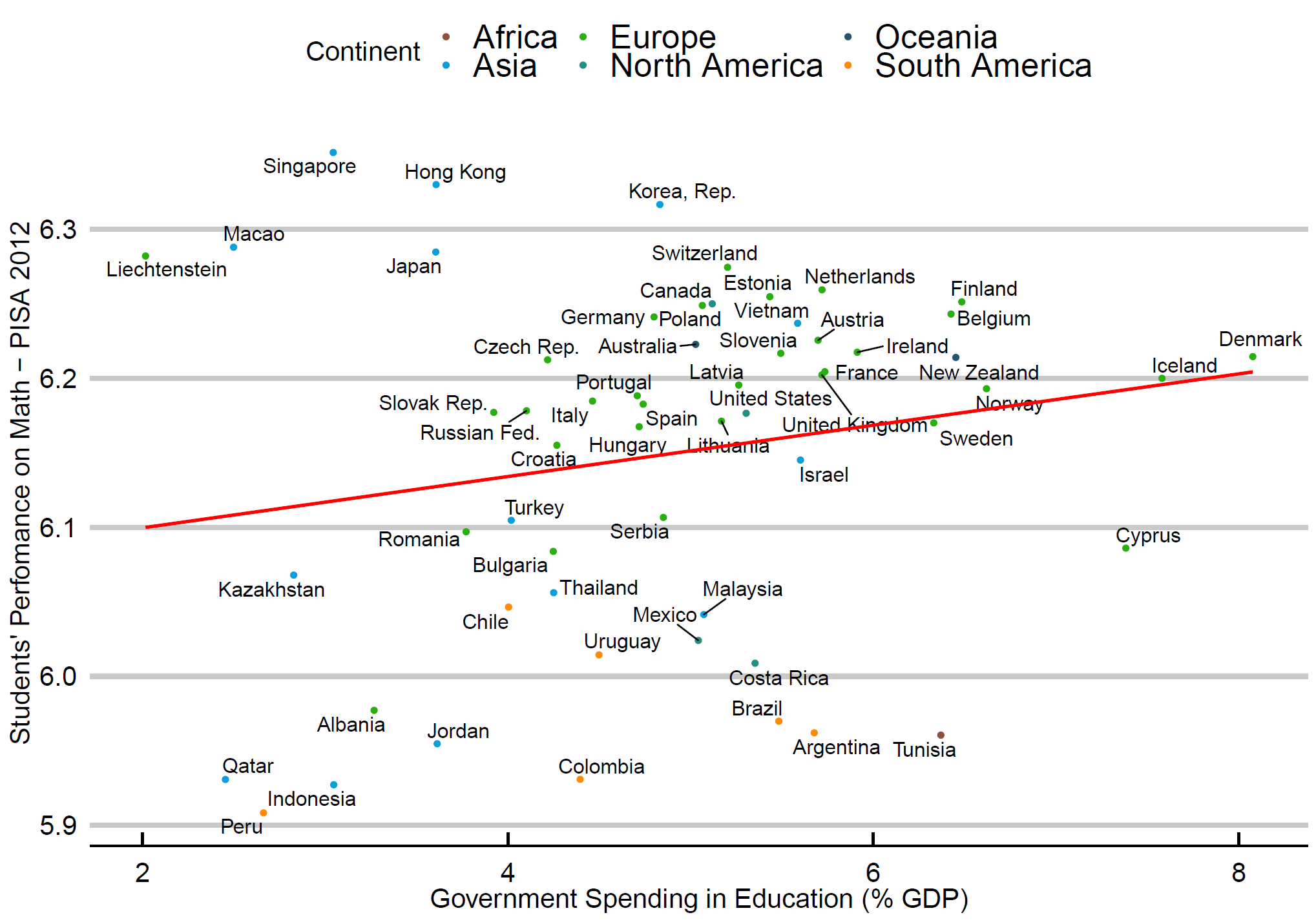
Create a scatterplot for each pair (Y,Xi) of your dataset. Are there outliers in your data?

# PISA score x Government Spending (%GDP)
p1 <- ggplot(PISA, aes(x=Gov_spend_educ, y=ln_score))
p1 <- p1 + geom_point(aes(color=Continent)) +  geom_text_repel(aes(label=Country), size=4.5)

p1<-p1+ stat_smooth(method = "lm", formula =y~x, se=FALSE, color="red") +
  scale_color_manual( values = c("#924F3E", "#099FDB", "#29B00E", "#208F84", "#23576E",  "darkorange"))+
  scale_x_continuous(name = "Government Spending in Education (% GDP)") +
  scale_y_continuous(name = "Students' Perfomance on Math - PISA 2012") +
  theme_economist_white(base_size = 17, gray_bg=FALSE)  
p1

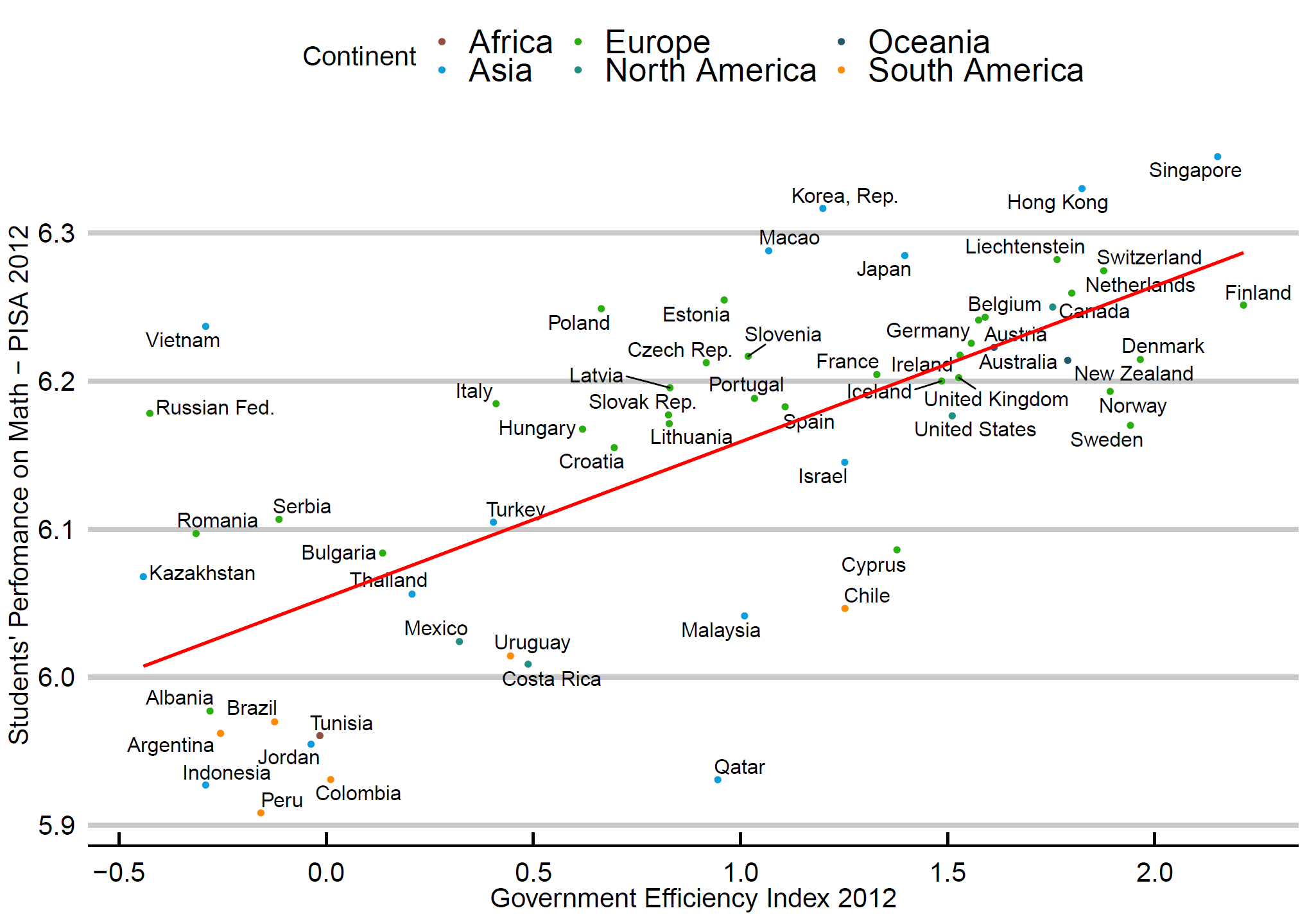
# PISA score x Government Efficiency Index
p2 <- ggplot(PISA, aes(x=Gov_Efficiency, y=ln_score))
p2 <- p2 + geom_point(aes(color=Continent)) +  geom_text_repel(aes(label=Country), size=4.5)

p2<-p2+ stat_smooth(method = "lm", formula =y~x, se=FALSE, color="red") +
  scale_color_manual( values = c("#924F3E", "#099FDB", "#29B00E", "#208F84", "#23576E",  "darkorange"))+
  scale_x_continuous(name = "Government Efficiency Index 2012") +
  scale_y_continuous(name = "Students' Perfomance on Math - PISA 2012") +
  theme_economist_white(base_size = 17, gray_bg=FALSE)  
p2

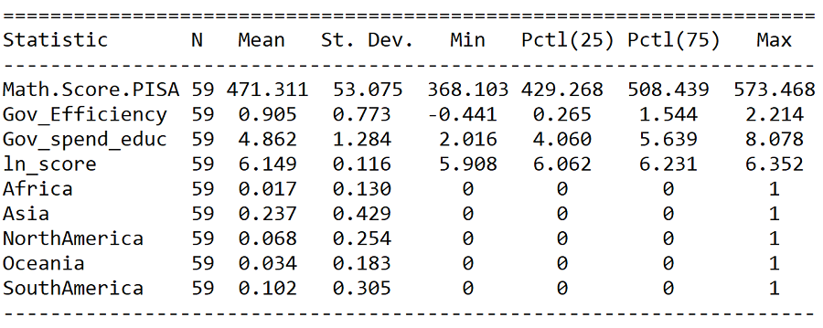
Step 2: Summary statistics

## Getting summary statistics with stargazer
stargazer(PISA, type="text")

Step 3: Run the full model and check assumptions

Run the model with all Xs in your dataset. Check the statistical significance - individual (t-test) and global (F-test). Then, check the model assumptions:

1. Normality
2. Homoskedasticity
3. Multicolinearity

##### Running the FULL MODEL

Full<-lm(ln_score~Gov_spend_educ+Gov_Efficiency+Africa+Asia+NorthAmerica+SouthAmerica+Oceania, data=PISA)
summary(Full)

# Use stargazer to get the regression table
stargazer(Full, type="text")

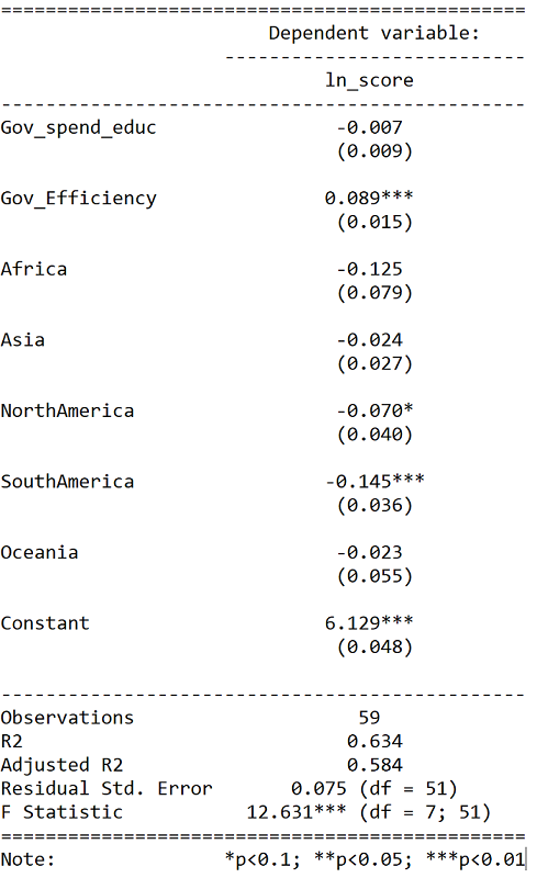
Only Gov_Efficiency and SouthAmerica are statistically significant at 5%. Therefore, your reduced model only includes those two independent variables.

## Checking the model assumptions
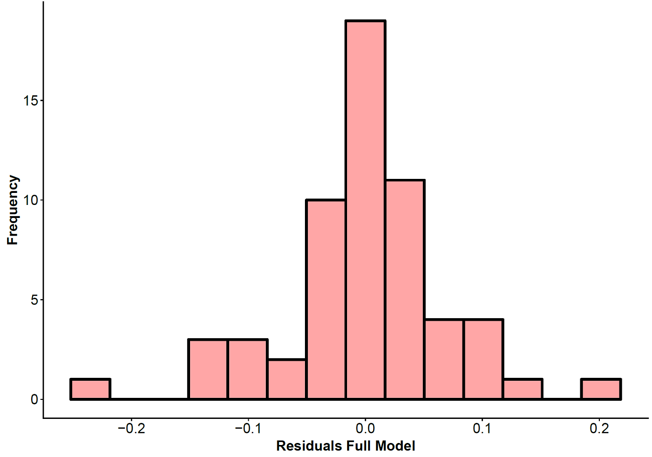
## Normality
resid_full<-as.data.frame(Full$residuals)
names(resid_full)[1]<-"resid"
hist_full <- ggplot(resid_full, aes(x = resid)) +
  geom_histogram(bins=14, position = "stack", size=1.5, col="black" ,fill = "#ff4d4d", alpha = 0.5) + labs(x = "Residuals Full Model", y="Frequency")+ theme(axis.text=element_text(size=18),axis.title=element_text(size=18,face="bold"), plot.title = element_text(size = 20, face = "bold"))
hist_full

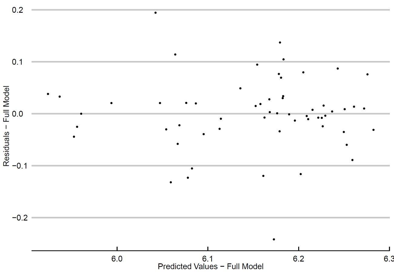
## Homoskedasticity
# First you need a dataframe with residuals and predicted values

predicted_full<-as.data.frame(Full$fitted.values)
names(predicted_full)[1]<-"pred"

homosk_full<-cbind(resid_full, predicted_full)

p3 <- ggplot(homosk_full, aes(x=pred, y=resid)) + geom_point()
p3 <- p3 +scale_x_continuous(name = "Predicted Values - Full Model") +
  scale_y_continuous(name = "Residuals - Full Model") +
  theme_economist_white(base_size = 17, gray_bg=FALSE)  
p3

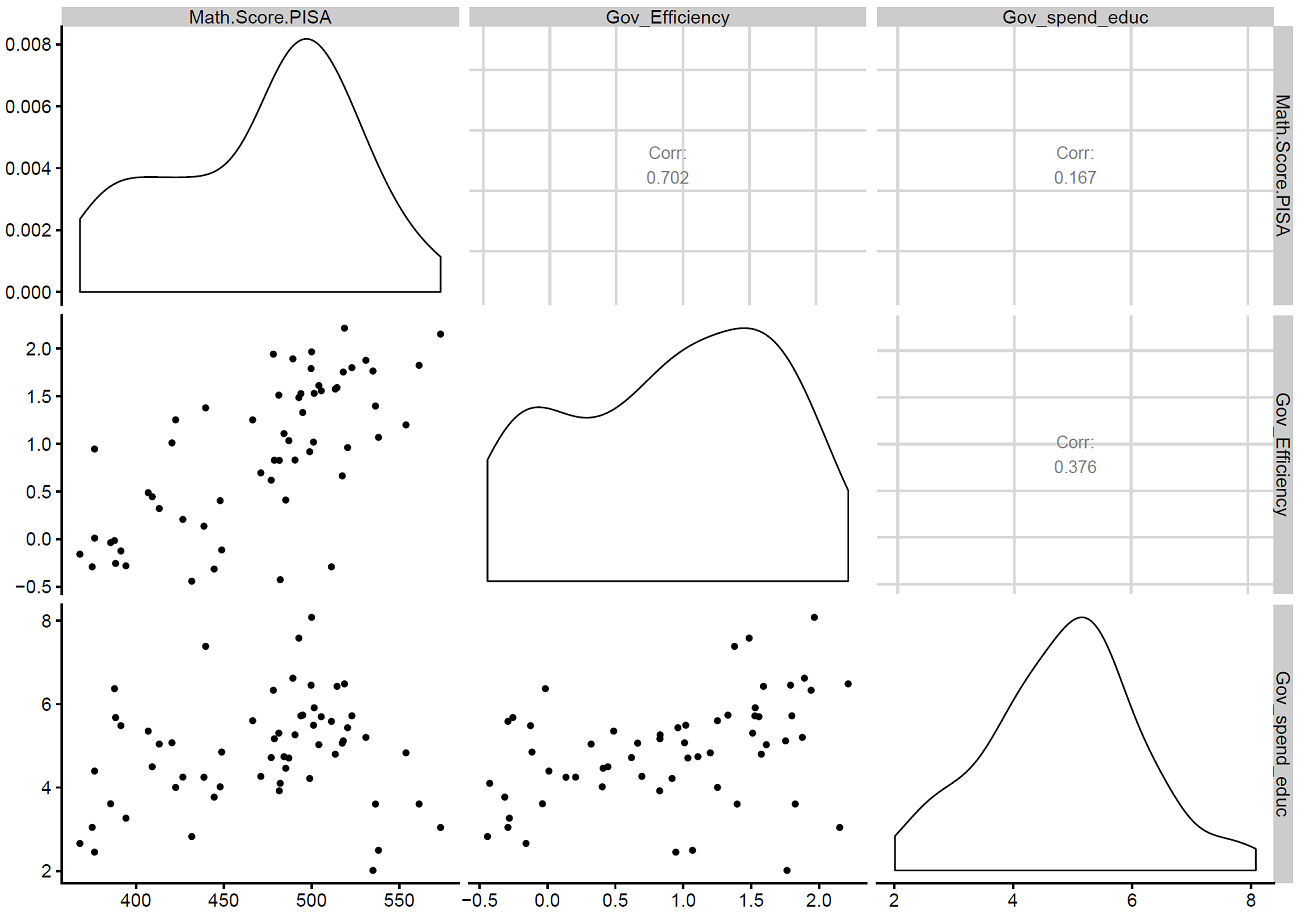
## Correlation Matrix
ggpairs(PISA[c(2:4)])

Step 4: Run the reduced model and check assumptions

Run the regression with Government Efficiency and SouthAmerica. Then, redo the visual inspection to check normality and homoskedasticity.

##### Running the REDUCED MODEL

Reduc<-lm(ln_score~Gov_Efficiency+SouthAmerica, data=PISA)
summary(Reduc)

# Use stargazer to get the regression table
stargazer(Reduc, type="text")

## Checking the model assumptions
## Normality
resid_reduc<-as.data.frame(Reduc$residuals)
names(resid_reduc)[1]<-"resid"
hist_reduc <- ggplot(resid_reduc, aes(x = resid)) +
  geom_histogram(bins=14, position = "stack", size=1.5, col="black" ,fill = "#ff4d4d", alpha = 0.5) + labs(x = "Residuals Reduced Model", y="Frequency")+ theme(axis.text=element_text(size=18),axis.title=element_text(size=18,face="bold"), plot.title = element_text(size = 20, face = "bold"))
hist_reduc

## Homoskedasticity

predicted_reduc<-as.data.frame(Reduc$fitted.values)
names(predicted_reduc)[1]<-"pred"

homosk_reduc<-cbind(resid_reduc, predicted_reduc)

p4 <- ggplot(homosk_reduc, aes(x=pred, y=resid)) + geom_point()
p4 <- p4 +scale_x_continuous(name = "Predicted Values - Reduced Model") +
  scale_y_continuous(name = "Residuals - Reduced Model") +
  theme_economist_white(base_size = 17, gray_bg=FALSE)  
p4

Step 5: Partial F-test

The last step is the Partial F-test. Remember: if you reject the null, use the full model. Otherwise, use the reduced model.

############################# Partial F-test
anova(Full, Reduc)
#### P-value = 0.28. Using an alfa=.05, I do not reject the null and
#### I will use the reduced model