8 Synthetic Control
8.1 Preliminaries
Here we replicate some results from Abadie, Diamond and Hainmueller (2015). Results are similar but not the same since I ignore the cross-validation exercise to choose the v weights. Nevertheless, conclusions remain the same. Original replication files can be found here.
Download the dataset germany.RDS here, and check lecture notes for discussion here.
8.2 The Economic Cost of the 1990 German Reunification
setwd("C:/Users/User/Desktop/474-Rlab/datasets")
data<-readRDS("germany.RDS")library(tidyverse)
library(Synth)
dataprep.out <-
dataprep(foo = data,
predictors = c("gdp","trade","infrate"),
predictors.op = "mean",
time.predictors.prior = 1960:1990,
dependent = "gdp",
unit.variable = "index",
unit.names.variable="country",
special.predictors = list(
list("industry" ,1981:1990, c("mean")),
list("schooling",c(1980,1985), c("mean")),
list("invest80" ,1980, c("mean"))),
time.variable = "year",
treatment.identifier = 7,
controls.identifier = c(1,2,3,4,5,6,8,9,10,12,14,16,18,19,20,21),
time.optimize.ssr = 1960:1990,
time.plot = 1960:2003
)synth.out <- synth(dataprep.out)synth.tables <- synth.tab(dataprep.res = dataprep.out,
synth.res = synth.out)
synth.tables## $tab.pred
## Treated Synthetic Sample Mean
## gdp 8566.452 8555.490 7429.167
## trade 46.163 51.322 52.037
## infrate 3.368 4.889 7.412
## special.industry.1981.1990 34.538 34.531 33.794
## special.schooling.1980.1985 55.500 55.475 38.659
## special.invest80.1980 27.018 27.022 25.895
##
## $tab.v
## v.weights
## gdp 0.114
## trade 0.001
## infrate 0
## special.industry.1981.1990 0.428
## special.schooling.1980.1985 0.316
## special.invest80.1980 0.14
##
## $tab.w
## w.weights unit.names unit.numbers
## 1 0.148 USA 1
## 2 0.049 UK 2
## 3 0.494 Austria 3
## 4 0.004 Belgium 4
## 5 0.004 Denmark 5
## 6 0.004 France 6
## 8 0.004 Italy 8
## 9 0.005 Netherlands 9
## 10 0.005 Norway 10
## 12 0.180 Switzerland 12
## 14 0.086 Japan 14
## 16 0.003 Greece 16
## 18 0.002 Portugal 18
## 19 0.002 Spain 19
## 20 0.005 Australia 20
## 21 0.004 New Zealand 21
##
## $tab.loss
## Loss W Loss V
## [1,] 3.990274e-05 8881.752library(kableExtra)
weights<-data.frame(synth.tables$tab.w)
weights<-weights%>%select(-unit.numbers)
names(weights)<-c("Weight", "Country")
kbl(weights, digits=2, caption = "Weights Table", booktabs = T) %>%
kable_styling(bootstrap_options = c("striped", "condensed"))balance<-synth.tables$tab.pred
rownames(balance)<-c("GDP per capita", "Trade openness", "Inflation rate", "Industry share", "Schooling", "Investment rate")
kbl(balance, digits=2, caption = "Balance Table 1960-2003", booktabs = T) %>%
kable_styling(bootstrap_options = c("striped", "condensed"))| Treated | Synthetic | Sample Mean | |
|---|---|---|---|
| GDP per capita | 8566.45 | 8555.49 | 7429.17 |
| Trade openness | 46.16 | 51.32 | 52.04 |
| Inflation rate | 3.37 | 4.89 | 7.41 |
| Industry share | 34.54 | 34.53 | 33.79 |
| Schooling | 55.50 | 55.48 | 38.66 |
| Investment rate | 27.02 | 27.02 | 25.90 |
path.plot(synth.res = synth.out, dataprep.res = dataprep.out,
          Ylab = "Per capita GDP (PPP, 2002 USD)", Xlab = "Year",
          Ylim = c(0, 35000), Legend = c("West Germany","Synthetic West Germany"), Legend.position = "bottomright",
          tr.intake = 1990)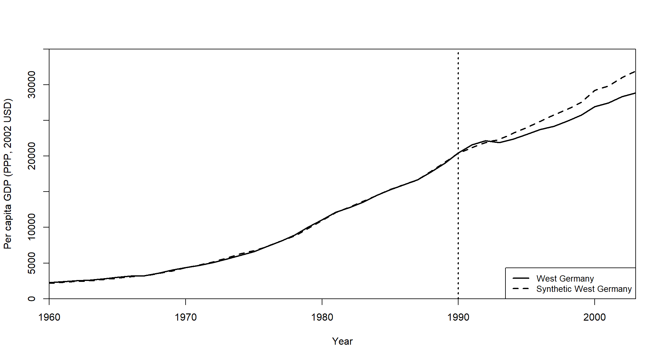
gaps.plot(synth.res = synth.out, dataprep.res = dataprep.out,
           Ylab = "Per capita GDP (PPP, 2002 USD)", Xlab = "Year",
          tr.intake = 1990)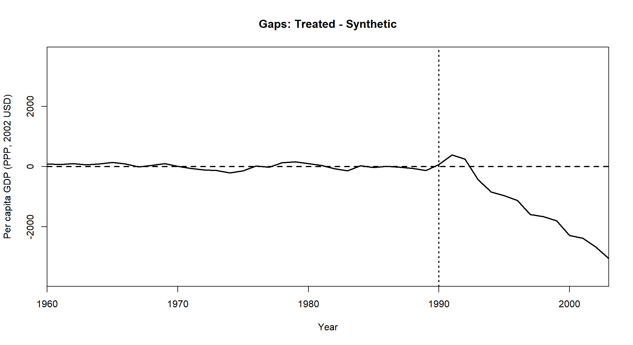
8.3 Placebo Studies
dataprep.out2 <-
  dataprep(foo = data,
           predictors    = c("gdp","trade","infrate"),
           predictors.op = "mean",
           time.predictors.prior = 1960:1975,
           dependent     = "gdp",
           unit.variable = "index",
           unit.names.variable="country",
           special.predictors = list(
           list("industry" ,1971:1975, c("mean")),
           list("schooling",c(1970,1975), c("mean")),
           list("invest80" ,1980, c("mean"))),
           time.variable = "year",
           treatment.identifier = 7,
           controls.identifier = c(1,2,3,4,5,6,8,9,10,12,14,16,18,19,20,21),
           time.optimize.ssr = 1960:1975,
           time.plot = 1960:1990
         )
synth.out2 <- synth(dataprep.out2)
path.plot(synth.res = synth.out2, dataprep.res = dataprep.out2,
          Ylab = "Per capita GDP (PPP, 2002 USD)", Xlab = "Year",
          Ylim = c(0, 35000), Legend = c("West Germany","Synthetic West Germany"), Legend.position = "bottomright",
          tr.intake = 1975)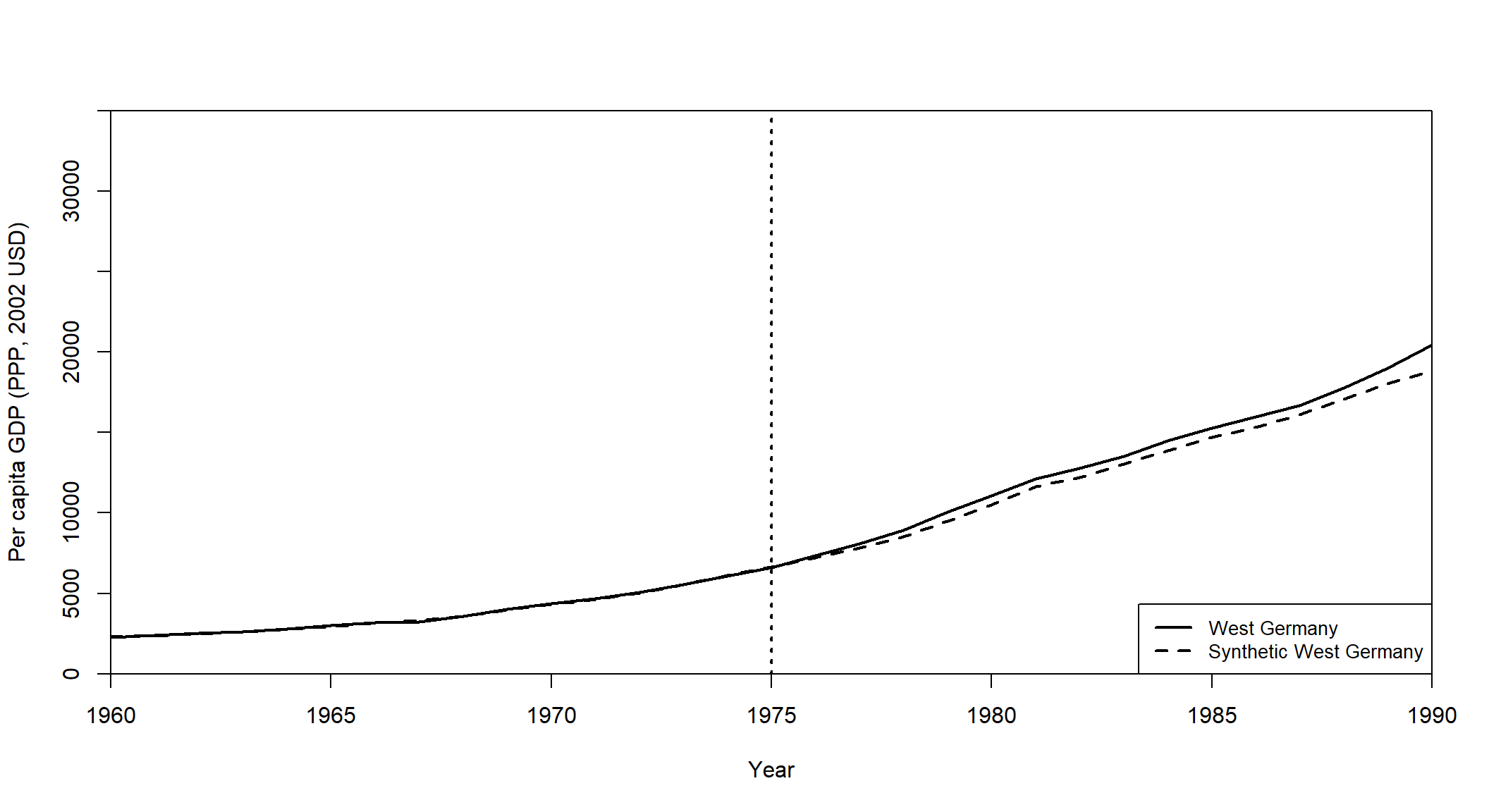
library(SCtools)
placebo <- generate.placebos(dataprep.out = dataprep.out,
synth.out = synth.out, strategy = "multiprocess")plot_placebos(placebo)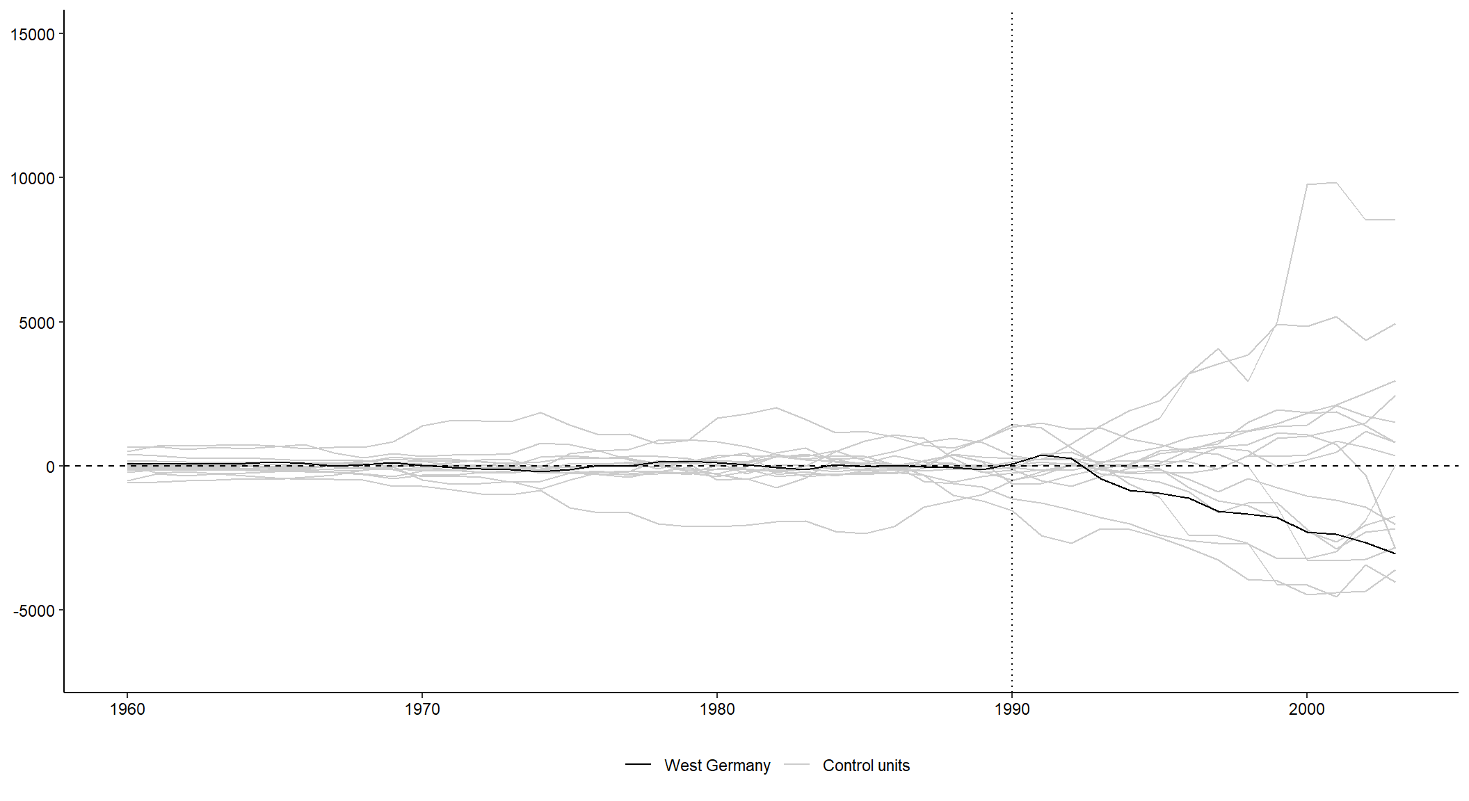
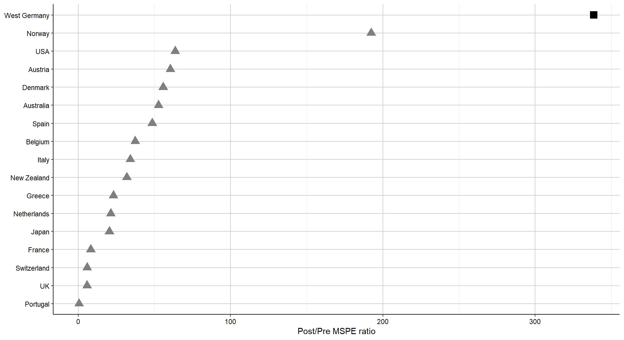
test_out <- mspe.test(placebo)
test_out$p.val
## [1] 0.05882353mspe.plot(tdf = placebo)