7 Difference-in-Differences
7.1 Line plots
The main identification assumption in the DinD framework is common trends. One way to see whether the assumption is reasonable in your setting is through line plots. The first step is to show how the outcomes in both treatment and control groups evolve - preferable with multiple pre-intervention periods.
Let’s replicate Figure 5.2 from Angrist and Pischke (2014) and see how trends in bank failures in Mississippi evolved before, during, and after the Caldwell crisis. Download the data here. In this exercise, we use the packages ggplot2 and ggthemes.
# If you don't have the packages, start with install.packages("ggplot2") and install.packages("ggthemes")
library(ggplot2)
library(ggthemes)

banks<-readRDS("banks.RDS")

plot1<-ggplot()+
  geom_line(data=banks, aes(x=year, y=`6th district`),size=1.4, color="#336666")+
  geom_line(data=banks, aes(x=year, y=`8th district`),size=1.4, color="#8abbd0")+
  labs(x = "Year", y="Number of banks in business")+
  theme_economist(base_size = 14) +
  scale_colour_economist()+
   theme(axis.text=element_text(size=12),
        axis.title=element_text(size=12,face="bold"))

plot1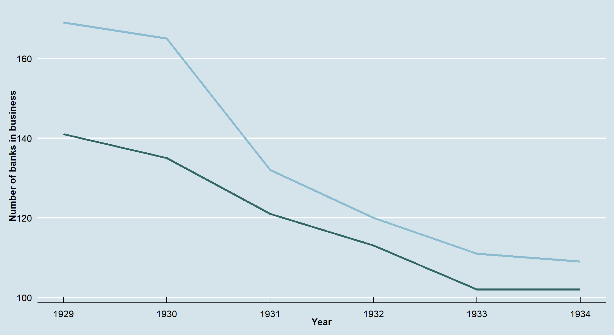
Instead of using geom_line() for each district, you can reshape the dataset. That will easily allow you to have legends for each line:
library(reshape2)
panel_banks<-melt(banks, id.var='year')
head(panel_banks,5)
## year variable value
## 1 1929 6th district 141
## 2 1930 6th district 135
## 3 1931 6th district 121
## 4 1932 6th district 113
## 5 1933 6th district 102Then, you apply almost the same code and get the plot with legends:
plot2<-ggplot()+
  geom_line(data=panel_banks, aes(x=year, y=value, col=variable),size=1.4)+
  scale_color_manual("", values=c("#8abbd0", "#336666"))+
  labs(x = "Year", y="Number of banks in business")+
  theme_economist(base_size = 14) +
  theme(axis.text=element_text(size=12),
      axis.title=element_text(size=12,face="bold"))
plot2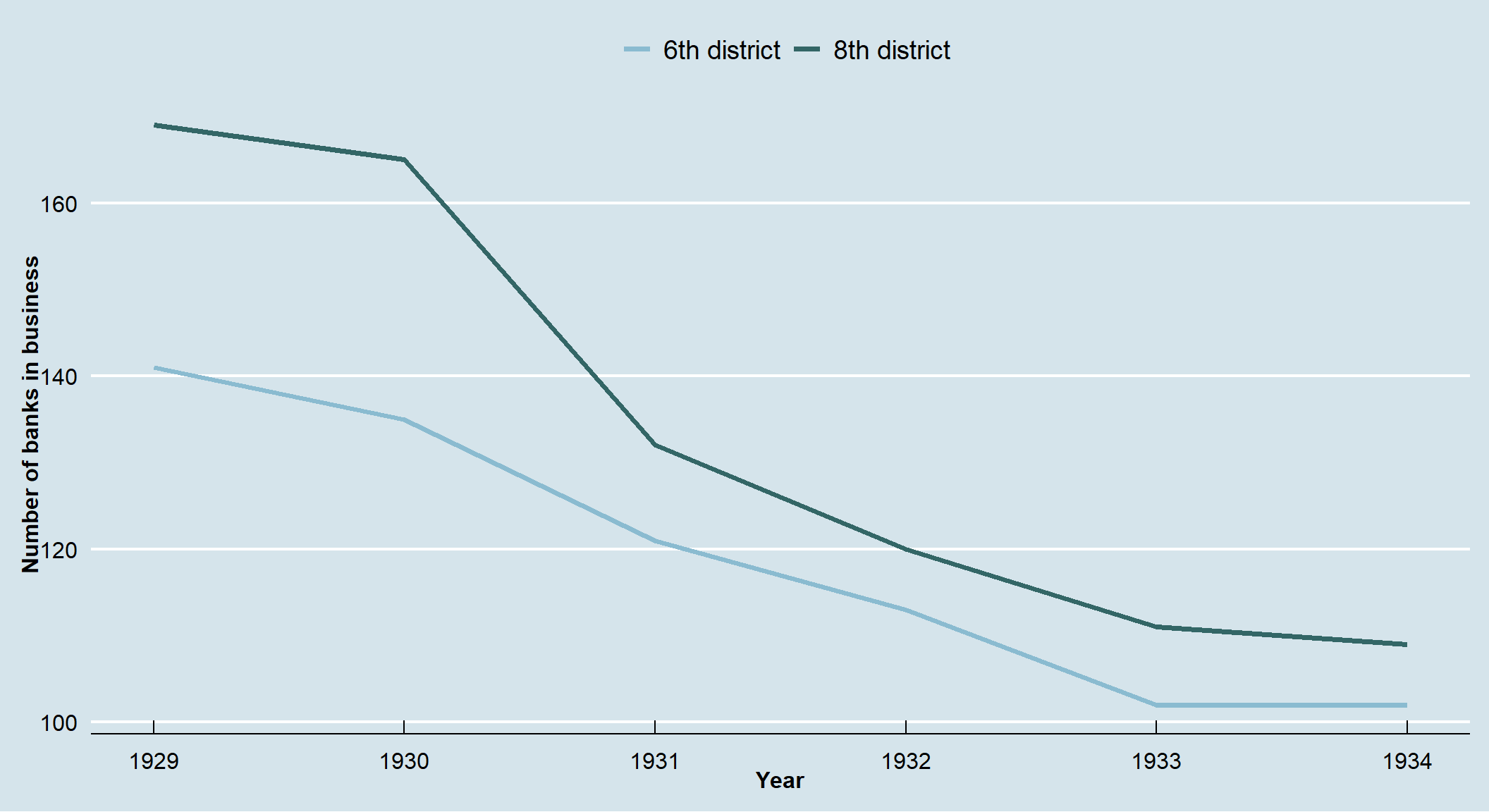
ggplot2 allows you to customize your graphs in many ways. For example, if you want different line types:
plot3<-ggplot()+
  geom_line(data=panel_banks, aes(x=year, y=value, col=variable, linetype = variable),size=1.4)+
  scale_color_manual("", values=c("#8abbd0", "#336666"))+
  scale_linetype_manual("", values = c("solid", "dashed"))+
  labs(x = "Year", y="Number of banks in business")+
  theme_economist(base_size = 14) +
  theme(axis.text=element_text(size=12),
      axis.title=element_text(size=12,face="bold"))
plot3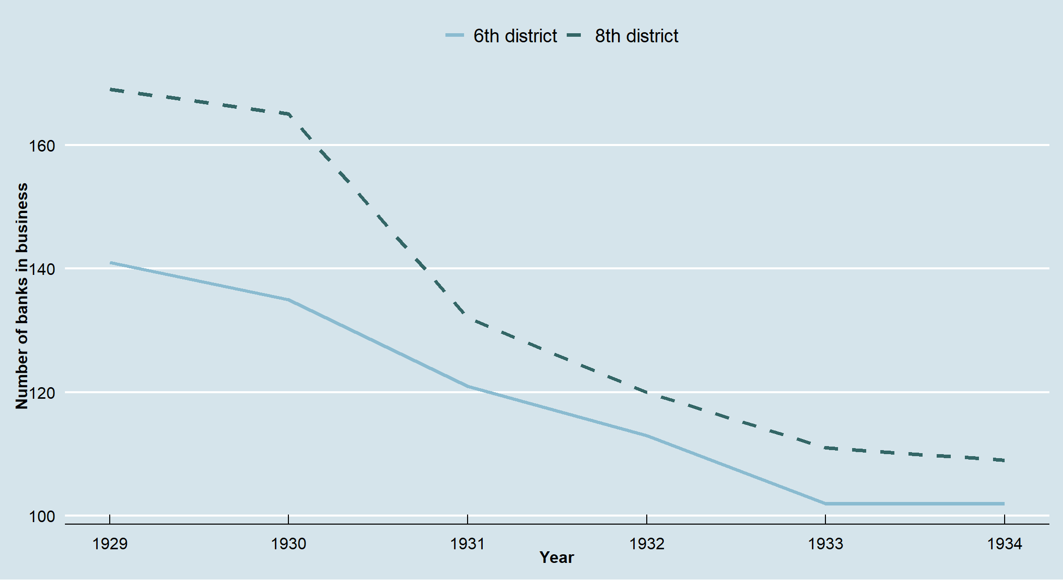
Check also ggthemes here. There you have plenty of options for the plot background.
7.2 2x2 Difference-in-Differences
TBD
7.3 Cheng and Hoekstra (2013)
These notes are mostly based on Cunningham (2021). This exercise replicates some of the results of Cheng and Hoekstra (2013). The dataset (download here) comprehends 50 U.S states during the period 2000-2010. The authors aimed to evaluate the effect of the staggered adoption of “stand your ground” laws on crime. Check lecture notes for discussion here.
The variables are described below:
| Variable | Definition |
|---|---|
| state | U.S. State |
| year | Year |
| region | Census Region. 1 if northeast, 2 if midwest, 3 if south and 4 if west |
| treated | 1 if state is treated at any point from 2000 and 2010 |
| cdl | Treatment variable. Takes values from 0 to 1, depending on which month of the year the new law was passed |
| l_motor | Motor theft rate (in log) |
| l_larceny | Larceny rate (in log) |
| l_robbery | Robbery rate (in log) |
| l_assault | Aggravated Assault rate (in log) |
| l_homicide | Murder rate (in log) |
| blackm_15_24 | % of black male aged 15-24 |
| whitem_15_24 | % of white male aged 15-24 |
| blackm_25_44 | % of black male aged 25-44 |
| whitem_25_44 | % of white male aged 25-44 |
| l_exp_subsidy | Government spending (assistance and subsidies) per capita (in log) |
| l_exp_pubwelfare | Government spending (public welfare) per capita (in log) |
| l_police | Police per 100,000 residents (in log) |
| unemployrt | Unemployment Rate (%) |
| poverty | Poverty Rate (%) |
| l_income | Median Household Income ($) (in log) |
| l_prisoner | Prisoners per 100,000 residents (in log) |
| l_lagprisoner | Lag prisoners per 100,000 residents (in log) |
| popwt | State Population (used in the weighted regression) |
7.3.1 Falsification tests
Intuitively, we would think think that the passing of the Castle-doctrine law would mainly affect a state’s homicide rate or level of crimes related to physically harming others. Whereas we would expect crimes like motor vehicle left and larceny to remain constant through the passing and implementation of the law. To test this assumption do the following regression analyses:
castle<-readRDS("castle.RDS")
library(fixest)
library(tidyverse)
## TWFE
reg_motor1<-feols(l_motor~cdl|state+year, cluster=~state, data=castle)

## TWFE with Region-by-Year Fixed Effects
reg_motor2<-feols(l_motor~cdl|state+year+region^year, cluster=~state, data=castle)

## TWFE with Region-by-Year Fixed Effects, additional controls and State-Specific Linear Time trends
reg_motor3<-feols(l_motor~cdl+blackm_15_24+whitem_15_24+blackm_25_44+
              whitem_25_44+l_exp_subsidy+l_exp_pubwelfare+l_police+
              unemployrt+poverty+l_income+l_prisoner+l_lagprisoner+
              state:year
              |state+year+region^year, cluster=~state, data=castle)

etable(reg_motor1,reg_motor2,reg_motor3,signif.code = c("***"=0.01, "**"=0.05, "*"=0.10),   keep=c("cdl","blackm_15_24","whitem_15_24","blackm_25_44",
                     "whitem_25_44","l_exp_subsidy","l_exp_pubwelfare","l_police",
                     "unemployrt","poverty","l_income","l_prisoner","l_lagprisoner"))
## reg_motor1 reg_motor2 reg_motor3
## Dependent Var.: l_motor l_motor l_motor
##
## cdl 0.0766* (0.0413) 0.0138 (0.0450) -0.0037 (0.0367)
## blackm_15_24 -0.0952* (0.0487)
## whitem_15_24 0.0046 (0.0155)
## blackm_25_44 0.0593** (0.0285)
## whitem_25_44 -0.0031 (0.0069)
## l_exp_subsidy -0.0144 (0.0309)
## l_exp_pubwelfare -0.0527 (0.0703)
## l_police 0.0049 (0.0372)
## unemployrt -0.0340** (0.0152)
## poverty -0.0010 (0.0114)
## l_income -0.1193 (0.1288)
## l_prisoner -0.0066 (0.1831)
## l_lagprisoner -0.2187 (0.2102)
## Fixed-Effects: ---------------- --------------- ------------------
## state Yes Yes Yes
## year Yes Yes Yes
## region-year No Yes Yes
## ________________ ________________ _______________ __________________
## S.E.: Clustered by: state by: state by: state
## Observations 550 550 550
## R2 0.95815 0.96851 0.98604
## Within R2 0.02611 0.00085 0.55696
## ---
## Signif. codes: 0 '***' 0.01 '**' 0.05 '*' 0.1 ' ' 1Note: The first column only considers state and year FEs. The second column adds region-by-year fixed effects, and the third column adds time-varying covariates and state-specific trends. All regressions are weighted by state population.
reg_lar1<-feols(l_larceny~cdl|state+year, cluster=~state, data=castle)
reg_lar2<-feols(l_larceny~cdl|state+year+region^year, cluster=~state, data=castle)
reg_lar3<-feols(l_larceny~cdl+blackm_15_24+whitem_15_24+blackm_25_44+
              whitem_25_44+l_exp_subsidy+l_exp_pubwelfare+l_police+
              unemployrt+poverty+l_income+l_prisoner+l_lagprisoner+
              state:year
            |state+year+region^year, cluster=~state, data=castle)

etable(reg_lar1,reg_lar2,reg_lar3,signifCode = c("***"=0.01, "**"=0.05, "*"=0.10),   keep=c("cdl","blackm_15_24","whitem_15_24","blackm_25_44",
                     "whitem_25_44","l_exp_subsidy","l_exp_pubwelfare","l_police",
                     "unemployrt","poverty","l_income","l_prisoner","l_lagprisoner"))
## reg_lar1 reg_lar2 reg_lar3
## Dependent Var.: l_larceny l_larceny l_larceny
##
## cdl 0.0075 (0.0227) 0.0015 (0.0208) -0.0137 (0.0231)
## blackm_15_24 -0.0489 (0.0368)
## whitem_15_24 -0.0022 (0.0105)
## blackm_25_44 0.0492* (0.0230)
## whitem_25_44 0.0018 (0.0043)
## l_exp_subsidy -0.0056 (0.0144)
## l_exp_pubwelfare 0.0485 (0.0318)
## l_police -0.0203 (0.0179)
## unemployrt -0.0010 (0.0061)
## poverty 0.0033 (0.0073)
## l_income 0.0076 (0.0738)
## l_prisoner -0.1146 (0.0780)
## l_lagprisoner 0.0311 (0.0987)
## Fixed-Effects: --------------- --------------- ----------------
## state Yes Yes Yes
## year Yes Yes Yes
## region-year No Yes Yes
## ________________ _______________ _______________ ________________
## S.E.: Clustered by: state by: state by: state
## Observations 550 550 550
## R2 0.94217 0.96118 0.98078
## Within R2 0.00096 3.97e-5 0.50489
## ---
## Signif. codes: 0 '***' 0.001 '**' 0.01 '*' 0.05 '.' 0.1 ' ' 1From the above regression results we can see that regardless of the covariates we add, the affect the new law has on larceny and motor vehicle left is not statistically significant. This provides a well established baseline for our falsification tests.
7.3.2 Deterrence
Besides just testing if homicide rates change, we would also like to investigate if the Castle doctrine laws have a significant deterrent effect. In other words, if potential criminals know that their victims can legally shoot them in self-defense, does this knowledge decrease certain types of crime?
reg_rob1<-feols(l_robbery~cdl|state+year, cluster=~state, data=castle)
reg_rob2<-feols(l_robbery~cdl|state+year+region^year, cluster=~state, data=castle)
reg_rob3<-feols(l_robbery~cdl+blackm_15_24+whitem_15_24+blackm_25_44+
              whitem_25_44+l_exp_subsidy+l_exp_pubwelfare+l_police+
              unemployrt+poverty+l_income+l_prisoner+l_lagprisoner+
              state:year
            |state+year+region^year, cluster=~state, data=castle)

etable(reg_rob1,reg_rob2,reg_rob3,signifCode = c("***"=0.01, "**"=0.05, "*"=0.10),   keep=c("cdl","blackm_15_24","whitem_15_24","blackm_25_44",
                     "whitem_25_44","l_exp_subsidy","l_exp_pubwelfare","l_police",
                     "unemployrt","poverty","l_income","l_prisoner","l_lagprisoner"))
## reg_rob1 reg_rob2 reg_rob3
## Dependent Var.: l_robbery l_robbery l_robbery
##
## cdl 0.0448 (0.0331) 0.0320 (0.0426) 0.0267 (0.0303)
## blackm_15_24 -0.2014* (0.0845)
## whitem_15_24 0.0103 (0.0230)
## blackm_25_44 0.1625* (0.0735)
## whitem_25_44 -0.0121 (0.0109)
## l_exp_subsidy 0.0061 (0.0261)
## l_exp_pubwelfare -0.0798 (0.0718)
## l_police 0.0132 (0.0305)
## unemployrt -0.0101 (0.0103)
## poverty -0.0095 (0.0116)
## l_income 0.0391 (0.1221)
## l_prisoner 0.0453 (0.1845)
## l_lagprisoner -0.3073. (0.1576)
## Fixed-Effects: --------------- --------------- -----------------
## state Yes Yes Yes
## year Yes Yes Yes
## region-year No Yes Yes
## ________________ _______________ _______________ _________________
## S.E.: Clustered by: state by: state by: state
## Observations 550 550 550
## R2 0.98516 0.98620 0.99273
## Within R2 0.01156 0.00467 0.47609
## ---
## Signif. codes: 0 '***' 0.001 '**' 0.01 '*' 0.05 '.' 0.1 ' ' 1reg_aslt1<-feols(l_assault~cdl|state+year, cluster=~state, data=castle)
reg_aslt2<-feols(l_assault~cdl|state+year+region^year, cluster=~state, data=castle)
reg_aslt3<-feols(l_assault~cdl+blackm_15_24+whitem_15_24+blackm_25_44+
whitem_25_44+l_exp_subsidy+l_exp_pubwelfare+l_police+
unemployrt+poverty+l_income+l_prisoner+l_lagprisoner+
state:year
|state+year+region^year, cluster=~state, data=castle)
etable(reg_aslt1,reg_aslt2,reg_aslt3,signifCode = c("***"=0.01, "**"=0.05, "*"=0.10), keep=c("cdl","blackm_15_24","whitem_15_24","blackm_25_44",
"whitem_25_44","l_exp_subsidy","l_exp_pubwelfare","l_police",
"unemployrt","poverty","l_income","l_prisoner","l_lagprisoner"))## reg_aslt1 reg_aslt2 reg_aslt3
## Dependent Var.: l_assault l_assault l_assault
##
## cdl 0.0555 (0.0604) 0.0698 (0.0638) 0.0317 (0.0386)
## blackm_15_24 0.0895 (0.0681)
## whitem_15_24 -0.0456 (0.0346)
## blackm_25_44 -0.0567 (0.0343)
## whitem_25_44 0.0103 (0.0115)
## l_exp_subsidy -0.0096 (0.0260)
## l_exp_pubwelfare 0.0603 (0.0404)
## l_police 0.1029*** (0.0232)
## unemployrt 0.0097 (0.0083)
## poverty -0.0068 (0.0099)
## l_income 0.0120 (0.1117)
## l_prisoner -0.0065 (0.1441)
## l_lagprisoner -0.0126 (0.1377)
## Fixed-Effects: --------------- --------------- ------------------
## state Yes Yes Yes
## year Yes Yes Yes
## region-year No Yes Yes
## ________________ _______________ _______________ __________________
## S.E.: Clustered by: state by: state by: state
## Observations 550 550 550
## R2 0.94615 0.95273 0.98960
## Within R2 0.01076 0.01415 0.78305
## ---
## Signif. codes: 0 '***' 0.001 '**' 0.01 '*' 0.05 '.' 0.1 ' ' 1From these regression results we can conclude there is no effect on robbery or aggravated assault and burglary. As the results are statistically insignificant, we do not find a deterrent effect from the passing and implementation of Castle-doctrine laws.
7.3.3 Homicide in Florida
Before doing multistate homicide regression analysis, we can specifically look at the state of Florida to get an idea of the affect the Castle-Doctrine laws had on homicide rates.
To best do this, lets visualization homicide rates in Florida compared to a control group containing all states who did not pass a similar Castle-doctrine law between 2000 to 2010.
florida<-castle%>%filter(state=="Florida"|treated==0)
florida<-florida%>%mutate(treat=ifelse(state=="Florida","Florida","Control Group"))
plot<-florida%>%group_by(treat, year)%>%summarize(Homicide=mean(l_homicide))
library(ggthemes)
ggplot()+
geom_line(data=plot,
aes(x=year, y=Homicide, col=treat),
size=1.4)+
scale_color_fivethirtyeight("Treatment Status")+
theme_fivethirtyeight()+
labs(x = "Year", y="Homicide (in log)")+
geom_vline(xintercept = 2005, linetype="dashed")+
scale_x_continuous(breaks=c(2000, 2003, 2005, 2008, 2010))+
theme(axis.text=element_text(size=12),
axis.title=element_text(size=12,face="bold"))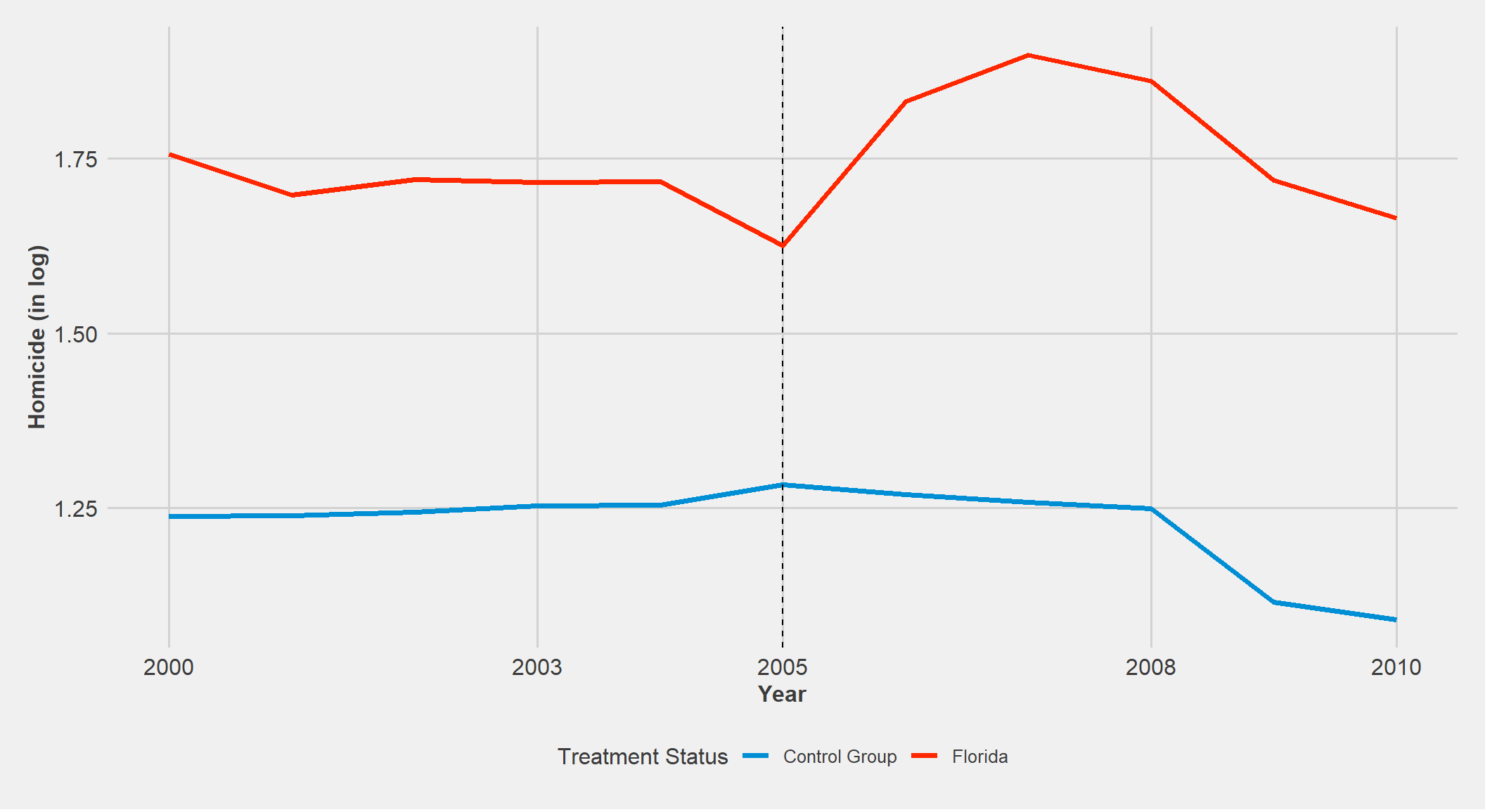 As shown in the graph, Florida starts with a higher average homicide rate than the control group, which decreases slightly (could be an issue with common trends). The homicide rate than increases substantially the years following 2005, then begins to return to its previous level around 2009. Whereas the control group’s homicide rate only decreases post 2005.
reg_homic1_fl<-feols(l_homicide~cdl|state+year, cluster=~state, data=florida)
reg_homic2_fl<-feols(l_homicide~cdl|state+year+region^year, cluster=~state, data=florida)
reg_homic3_fl<-feols(l_homicide~cdl+blackm_15_24+whitem_15_24+blackm_25_44+
                  whitem_25_44+l_exp_subsidy+l_exp_pubwelfare+l_police+
                  unemployrt+poverty+l_income+l_prisoner+l_lagprisoner+
                  state:year
                |state+year+region^year, cluster=~state, data=florida)

etable(reg_homic1_fl,reg_homic2_fl,reg_homic3_fl,signif.code = c("***"=0.01, "**"=0.05, "*"=0.10),   keep=c("cdl","blackm_15_24","whitem_15_24","blackm_25_44",
                     "whitem_25_44","l_exp_subsidy","l_exp_pubwelfare","l_police",
                     "unemployrt","poverty","l_income","l_prisoner","l_lagprisoner"))
## reg_homic1_fl reg_homic2_fl reg_homic3_fl
## Dependent Var.: l_homicide l_homicide l_homicide
##
## cdl 0.1376*** (0.0353) 0.0457 (0.1134) 0.2674** (0.1192)
## blackm_15_24 -0.0366 (0.1948)
## whitem_15_24 0.1264 (0.0793)
## blackm_25_44 0.0710 (0.1585)
## whitem_25_44 -0.0496*** (0.0164)
## l_exp_subsidy 0.0530 (0.0607)
## l_exp_pubwelfare 0.4054** (0.1766)
## l_police 0.2374 (0.3583)
## unemployrt 0.0489** (0.0227)
## poverty -0.0706** (0.0334)
## l_income -0.6636* (0.3297)
## l_prisoner -1.034*** (0.3533)
## l_lagprisoner 0.1821 (0.3755)
## Fixed-Effects: ------------------ --------------- -------------------
## state Yes Yes Yes
## year Yes Yes Yes
## region-year No Yes Yes
## ________________ __________________ _______________ ___________________
## S.E.: Clustered by: state by: state by: state
## Observations 330 330 330
## R2 0.91563 0.92657 0.95739
## Within R2 0.00515 0.00057 0.42002
## ---
## Signif. codes: 0 '***' 0.01 '**' 0.05 '*' 0.1 ' ' 1To put numbers to our visualization we run a regression like we have before. A large but only slightly significant affect on homicide rate can be found after adding all our covariates.
florida_plot = feols(l_homicide~i(year, treated, ref=2004)|state+year, cluster=~state, data=florida)
#coefplot(florida_plot)
iplot(florida_plot, main="Effect of Castle Doctrine on Homicide rates in Florida")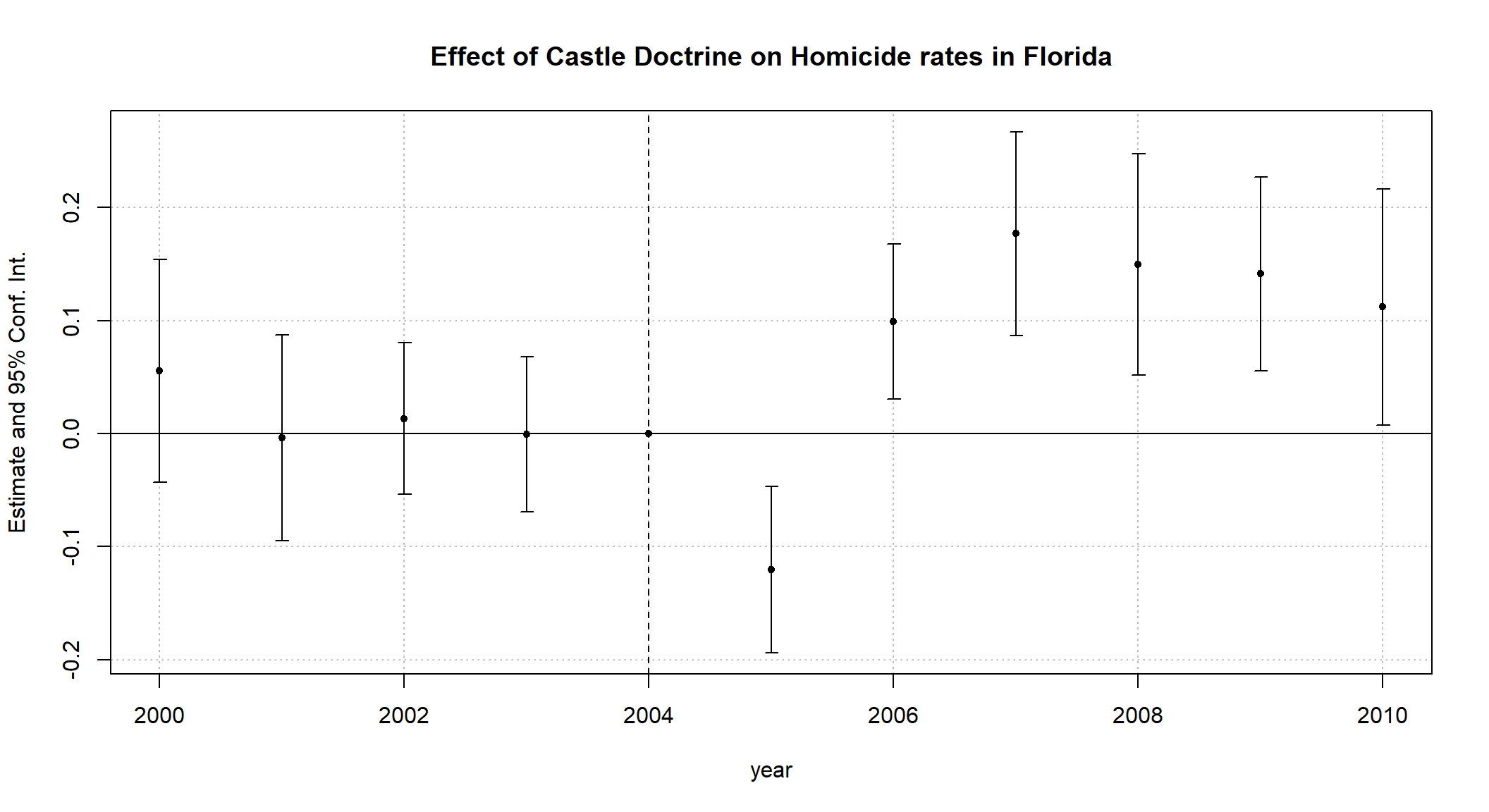 The above graph plots confidence intervals alongside the point estimates that we had found for each year. By doing this, we get a better understanding of how confident we in the affect Castle-doctrine laws have on each years homicide rates. In this case, all years post 2005 have a statistically significant increase as all of the confidence intervals do not include zero.
7.3.4 Multistate Homicide Regression
reg_homic1<-feols(l_homicide~cdl|state+year, cluster=~state, data=castle)
reg_homic2<-feols(l_homicide~cdl|state+year+region^year, cluster=~state, data=castle)
reg_homic3<-feols(l_homicide~cdl+blackm_15_24+whitem_15_24+blackm_25_44+
                     whitem_25_44+l_exp_subsidy+l_exp_pubwelfare+l_police+
                     unemployrt+poverty+l_income+l_prisoner+l_lagprisoner+
                     state:year
                   |state+year+region^year,cluster=~state, data=castle)

etable(reg_homic1,reg_homic2,reg_homic3,signifCode = c("***"=0.01, "**"=0.05, "*"=0.10),
       keep=c("cdl","blackm_15_24","whitem_15_24","blackm_25_44",
                     "whitem_25_44","l_exp_subsidy","l_exp_pubwelfare","l_police",
                     "unemployrt","poverty","l_income","l_prisoner","l_lagprisoner"))
## reg_homic1 reg_homic2 reg_homic3
## Dependent Var.: l_homicide l_homicide l_homicide
##
## cdl 0.0877 (0.0638) 0.0811 (0.0779) 0.0672 (0.0457)
## blackm_15_24 0.0984 (0.1269)
## whitem_15_24 0.0676. (0.0401)
## blackm_25_44 0.1195 (0.1358)
## whitem_25_44 -0.0375** (0.0133)
## l_exp_subsidy -0.0686 (0.0595)
## l_exp_pubwelfare 0.0645 (0.1059)
## l_police 0.1465* (0.0643)
## unemployrt 0.0196 (0.0189)
## poverty -0.0488* (0.0222)
## l_income -0.5859* (0.2803)
## l_prisoner -0.1407 (0.3372)
## l_lagprisoner -0.2033 (0.3975)
## Fixed-Effects: --------------- --------------- ------------------
## state Yes Yes Yes
## year Yes Yes Yes
## region-year No Yes Yes
## ________________ _______________ _______________ __________________
## S.E.: Clustered by: state by: state by: state
## Observations 550 550 550
## R2 0.91055 0.91527 0.95323
## Within R2 0.01308 0.00869 0.45273
## ---
## Signif. codes: 0 '***' 0.001 '**' 0.01 '*' 0.05 '.' 0.1 ' ' 1Finally, we can run a multistate homicide regression. Looking at the results of this regression we see the coefficient on cdl is not statistically significant. Therefore, we would think the Castle-doctrine would have no affect on homicide rates… However, we can add further complexity to the model to ensure are results are more accurate.
reg_homic1<-feols(l_homicide~cdl|state+year, cluster=~state,weights=castle$popwt, data=castle)
reg_homic2<-feols(l_homicide~cdl|state+year+region^year, weights=castle$popwt, cluster=~state, data=castle)
reg_homic3<-feols(l_homicide~cdl+blackm_15_24+whitem_15_24+blackm_25_44+
                     whitem_25_44+l_exp_subsidy+l_exp_pubwelfare+l_police+
                     unemployrt+poverty+l_income+l_prisoner+l_lagprisoner+
                     state:year
                   |state+year+region^year, weights=castle$popwt, cluster=~state, data=castle)

etable(reg_homic1,reg_homic2,reg_homic3,signifCode = c("***"=0.01, "**"=0.05, "*"=0.10),
       keep=c("cdl","blackm_15_24","whitem_15_24","blackm_25_44",
                     "whitem_25_44","l_exp_subsidy","l_exp_pubwelfare","l_police",
                     "unemployrt","poverty","l_income","l_prisoner","l_lagprisoner"))
## reg_homic1 reg_homic2 reg_homic3
## Dependent Var.: l_homicide l_homicide l_homicide
##
## cdl 0.0801* (0.0342) 0.0946** (0.0282) 0.1004* (0.0395)
## blackm_15_24 0.0613 (0.1089)
## whitem_15_24 0.0375 (0.0274)
## blackm_25_44 0.2302. (0.1263)
## whitem_25_44 -0.0283* (0.0120)
## l_exp_subsidy -0.0429 (0.0395)
## l_exp_pubwelfare 0.0494 (0.0644)
## l_police 0.1291* (0.0500)
## unemployrt 0.0142 (0.0121)
## poverty -0.0180 (0.0128)
## l_income -0.3152. (0.1643)
## l_prisoner -0.1367 (0.1953)
## l_lagprisoner -0.4096 (0.2566)
## Fixed-Effects: ---------------- ----------------- -----------------
## state Yes Yes Yes
## year Yes Yes Yes
## region-year No Yes Yes
## ________________ ________________ _________________ _________________
## S.E.: Clustered by: state by: state by: state
## Observations 550 550 550
## R2 0.93417 0.94109 0.96239
## Within R2 0.03018 0.03020 0.38079
## ---
## Signif. codes: 0 '***' 0.001 '**' 0.01 '*' 0.05 '.' 0.1 ' ' 1The above regression adds weights to the regression to account for state population differences. After adding this aspect, we find a statistically significant impact on the increase in homicide rates coming from self defense laws. These results are significant regardless of the covariates that get added, but as the covariate count increases we see a larger impact on our outcome variable cdl.
7.3.5 Multistate Event-Study
TBD