class: center, middle, inverse, title-slide # Econ 474 - Econometrics of Policy Evaluation ## Regression Discontinuity Designs ### Marcelino Guerra ### April 20-27, 2022 --- <style type="text/css"> .pull-left2 { float: left; width: 43%; } .pull-right2 { float: right; width: 53%; } .pull-right2 ~ p { clear: both; } </style> <style type="text/css"> .pull-left3 { float: left; width: 53%; } .pull-right3 { float: right; width: 43%; } .pull-right3 ~ p { clear: both; } </style> <style type="text/css"> .pull-left4 { float: left; width: 37%; } .pull-right4 { float: right; width: 60%; } .pull-right4 ~ p { clear: both; } </style> # Introduction * Regression Discontinuity (RD) Designs exploits rules that constraint the role of chance in human affairs - some rules are arbitrary and therefore provide a good experiment * For instance, the minimum legal drinking age, limits for school class size, social security full retirement age, voting system, among others -- * The method is based on a simple, intuitive idea: around the cutoff, the treatment might be as good as random so that one can compare units just above and below that threshold `$$\text{Rules} \rightarrow \text{Cutoffs} \rightarrow \text{Treatment Status}$$` -- * RD comes in two styles: sharp and fuzzy * The Sharp RD can be seen as a selection-on-observables story * The Fuzzy RD leads to an IV type of framework * Just as the Synthetic Control, RD is a very picture-intensive method --- class: inverse, middle, center # Sharp RD Design: Minimum Legal Drinking Age (MLDA) --- # Birthdays and Funerals .pull-left[ * Two views * Set the minimum legal drinking age to 18 (Vietnam era threshold) to promote a culture of mature alcohol consumption * The age-21 MLDA reduces youth access to alcohol and prevents some harm * The MLDA story gives us two natural experiments * [Each U.S. state has enough discretion to set/change policies](https://guerramarcelino.github.io/Econ474/Lectures/Lec6/lec6?panelset6=did-regression3&panelset7=2x2-difference-in-differences2&panelset8=regression-results4&panelset9=did-assumptions2&panelset10=threats-to-validity2&panelset11=deterrence2#23) * A slight change in age generates a significant change in legal access to alcohol ] .pull-right[ 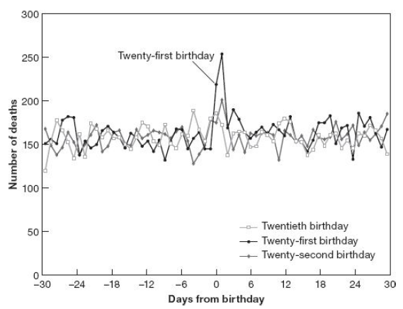 .small[**Note: The figure shows the number of deaths among Americans aged 20-22 between 1997 and 2003 .Source: Angrist and Pischke (2014).**] ] --- # MLDA Mortality Effects I .panelset[ .panel[.panel-name[Estimate of MLDA Mortality Effects] .pull-left[* The story linking the MLDA with a sharp and sustained rise in deaths is told in the Figure * Extrapolating the trend line drawn to the left of the cutoff (age 21), we would expect a death rate below 95 (the road not taken). Instead, the trend line on the right of the cutoff starts above 100 * What is the effect of legal access to alcohol on death rates? Using RD design, you answer this question by taking the difference in predicted values at the point of discontinuity between the two regressions ] .pull-right[ 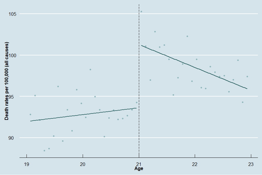 ] ] .panel[.panel-name[R code] ```r library(tidyverse) library(ggthemes) data("mlda", package = "masteringmetrics") mlda <- mutate(mlda, age = agecell - 21, over21 = ifelse(agecell >= 21,1,0)) ggplot(mlda, aes(x=agecell, y=all)) + geom_point(color="#91b8bd") + geom_smooth(aes(group=over21),method = "lm", formula =y~x, se=F, color="#336666") + scale_x_continuous(name = "Age") + scale_y_continuous(name = "Death rates per 100,000 (all causes)") + geom_vline(xintercept=21,linetype = "longdash" )+ theme_economist(base_size = 17)+ theme(axis.text=element_text(size=12), axis.title=element_text(size=12,face="bold")) ``` ] ] --- # MLDA Mortality Effects II .panelset[ .panel[.panel-name[Sharp RD] * To formalize the idea, set the treatment variable as `\(D_{a}\)`, where `\(D_{a}=1\)` indicates legal drinking and 0 otherwise. The treatment variable is a function of `\(a\)` - age. The MLDA transforms 21-year-olds from underage minors to legal alcohol consumers `$$D_{a} = \Bigg\{ \begin{array} & 1 & \text{if} & a \geq 21 \\ 0 & \text{if} & a < 21 \end{array}$$` * This highlights two features of RD designs: * `\(a\)` (the running variable) determines the treatment - once you know `\(a\)`, you know the treatment status `\(D_{a}\)` * The treatment status is a discontinuous function of `\(a\)`. In the sharp RD, the treatment switches on or off according to the cutoff ] .panel[.panel-name[Sharp RD Estimates] .pull-left[ The RD analysis of the MLDA estimates causal effects using the following: `$$\bar{M}_{a} = \alpha + \rho D_{a} + \gamma a + \varepsilon_{a}$$` where `\(\bar{M}_{a}\)` is the death rate in month `\(a\)`, `\(D_{a}\)` is the treatment status, and `\(a\)` is a linear control for age in months (from the twenty-first birthday). The parameter of interest `\(\rho\)` captures the jump in death rates at age 21. The equation above tells us that `\(D_{a}\)` is solely determined by `\(a\)`. Assuming also that the effect of `\(a\)` on death rates is captured by a linear function, we can be sure that there is no OVB left in this regression. ] .pull-right[ ``` ## reg ## Dependent Var.: all ## ## (Intercept) 91.84*** (0.7090) ## age -0.9747 (0.6639) ## over21 7.663*** (1.514) ## _______________ _________________ ## S.E. type Heteroskeda.-rob. ## Observations 48 ## R2 0.59456 ## Adj. R2 0.57654 ## --- ## Signif. codes: 0 '***' 0.001 '**' 0.01 '*' 0.05 '.' 0.1 ' ' 1 ``` ] ] .panel[.panel-name[R code] ```r library(fixest) reg<-feols(all~age+over21, se="hetero", data=mlda) etable(reg) ``` ] ] --- # RD Specifics I .panelset[ .panel[.panel-name[Linear x Nonlinear Relationship] .pull-left[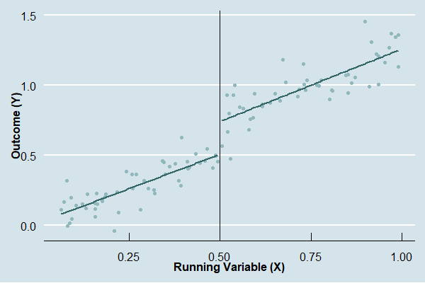] .pull-right[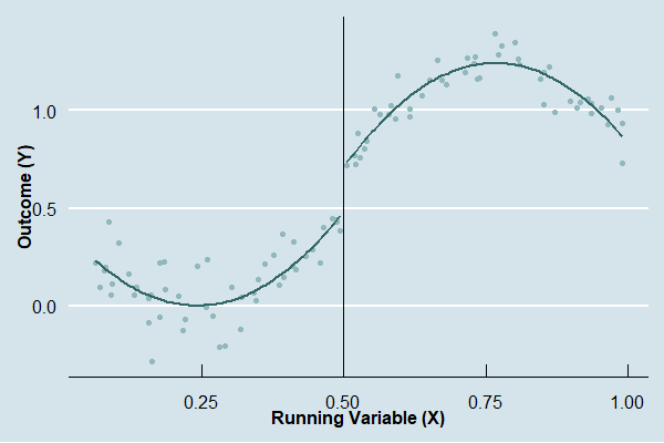] ] .panel[.panel-name[Nonlinearity mistaken for discontinuity] .pull-left[ When there is a nonlinear relationship, we can construct the RD estimates by fitting `$$Y_{i} = f(x_{i})+\rho D_{i} + \eta_{i}$$` where `\(f(a)\)` is continuous in a neighborhood of `\(x_{0}\)`. For instance, modeling `\(f(x_{i})\)` with a *p*th-order polinomial, you get RD estimates with `$$Y_{i}=\alpha+\beta_{1}x_{i}+\beta_{2}x^{2}_{i}+...+\beta_{p}x^{p}_{i}+\rho D_{i} + \eta_{i}$$` **Caution:** the figure highlights the challenge RD designers face. Here, the figure exhibits nonlinear trend, but no discontinuity. ] .pull-right[ 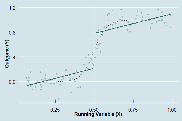] ] ] --- # MLDA Mortality Effects III .panelset[ .panel[.panel-name[Estimate of MLDA Mortality Effects] .pull-left[ There might be a mild curvature in the relationship between death rates and age, and one can model the RD with the quadratic running variable as `$$\bar{M}_{a} = \alpha + \rho D_{a} + \gamma_{1} a + \gamma_{2}a^{2} + \varepsilon_{a}$$` A related modification allows for different running variable coefficients to the left and right of the cutoff. The modification generates models that interact `\(a\)` with `\(D_{a}\)`. Nonlinear trends combined with interaction looks like `$$\bar{M}_{a} = \alpha + \rho D_{a} + \gamma_{1} a + \gamma_{2}a^{2} +\delta_{1}aD_{a}+\delta_{2}a^{2}D_{a} + \varepsilon_{a}$$` ] .pull-right[ 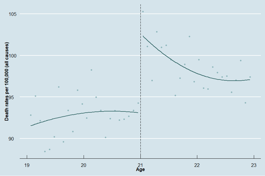 ] ] .panel[.panel-name[Regression results] .pull-left[ * In this setup, both the linear and quadratic terms change as we cross the cutoff * Just as in the linear case, `\(\rho\)` is the parameter of interest. Now, the estimate is around 9.5 deaths per 100,000 - larger than the linear case ] .pull-right[ ``` ## reg ## Dependent Var.: all ## ## (Intercept) 93.07*** (0.7799) ## poly(age,2,raw=TRUE)1 -0.8306 (2.850) ## poly(age,2,raw=TRUE)2 -0.8403 (1.541) ## over21 9.548*** (1.830) ## poly(age,2,raw=TRUE) x over211 -6.017 (4.528) ## poly(age,2,raw=TRUE) x over212 2.904 (2.257) ## ______________________________ _________________ ## S.E. type Heteroskeda.-rob. ## Observations 48 ## R2 0.68208 ## Adj. R2 0.64423 ## --- ## Signif. codes: 0 '***' 0.001 '**' 0.01 '*' 0.05 '.' 0.1 ' ' 1 ``` ] ] .panel[.panel-name[R code] ```r library(fixest) reg<-feols(all~poly(age, 2, raw = TRUE)*over21+over21, se="hetero", data=mlda) etable(reg) ``` ] ] --- # MLDA Mortality Effects IV .panelset[ .panel[.panel-name[Robustness] .pull-left[ 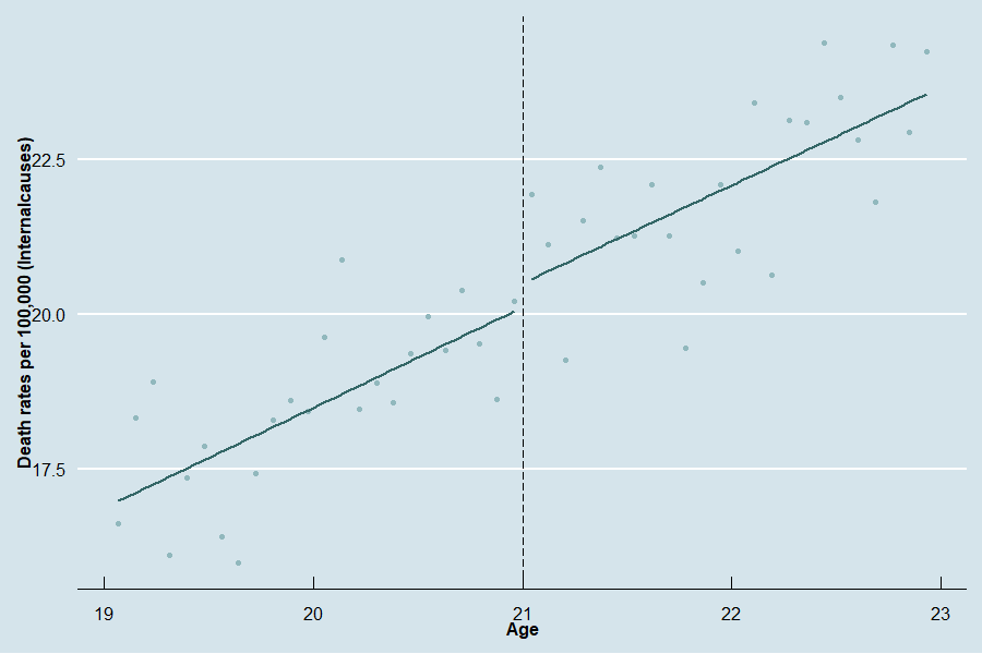 ] .pull-right[ 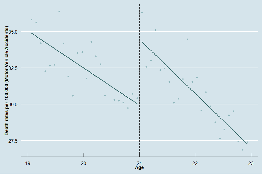] ] .panel[.panel-name[Regression results I] ``` ## reg1 reg2 ## Dependent Var.: internal internal ## ## (Intercept) 20.09*** (0.2730) 20.07*** (0.4900) ## age 1.600*** (0.2472) ## over21 0.3919 (0.5431) 1.073 (0.8015) ## poly(age,2,raw=TRUE)1 1.500 (1.340) ## poly(age,2,raw=TRUE)2 -0.0601 (0.6886) ## poly(age,2,raw=TRUE) x over211 -1.870 (2.015) ## poly(age,2,raw=TRUE) x over212 1.050 (0.9882) ## ______________________________ _________________ _________________ ## S.E. type Heteroskeda.-rob. Heteroskeda.-rob. ## Observations 48 48 ## R2 0.79935 0.80761 ## Adj. R2 0.79044 0.78471 ## --- ## Signif. codes: 0 '***' 0.001 '**' 0.01 '*' 0.05 '.' 0.1 ' ' 1 ``` ] .panel[.panel-name[Regression results II] ``` ## reg3 reg4 ## Dependent Var.: mva mva ## ## (Intercept) 29.36*** (0.3409) 29.81*** (0.4869) ## age -3.149*** (0.3095) ## over21 4.534*** (0.7173) 4.663*** (1.093) ## poly(age,2,raw=TRUE)1 -2.933. (1.625) ## poly(age,2,raw=TRUE)2 -0.1852 (0.8247) ## poly(age,2,raw=TRUE) x over211 -0.8231 (2.730) ## poly(age,2,raw=TRUE) x over212 0.1985 (1.304) ## ______________________________ __________________ _________________ ## S.E. type Heteroskedas.-rob. Heteroskeda.-rob. ## Observations 48 48 ## R2 0.70255 0.72244 ## Adj. R2 0.68933 0.68939 ## --- ## Signif. codes: 0 '***' 0.001 '**' 0.01 '*' 0.05 '.' 0.1 ' ' 1 ``` ] .panel[.panel-name[R code] ```r library(fixest) reg1<-feols(internal~age+over21, se="hetero", data=mlda) reg2<-feols(internal~poly(age, 2, raw = TRUE)*over21+over21, se="hetero", data=mlda) reg3<-feols(mva~age+over21, se="hetero", data=mlda) reg4<-feols(mva~poly(age, 2, raw = TRUE)*over21+over21, se="hetero", data=mlda) etable(reg1,reg2,reg3,reg4) ``` ] ] --- # RD Specifics II * A second RD strategy exploits the fact that we are not concerned about nonlinear trends for the small set of points very close to the cutoff so that one can compare averages in a narrow window just to the left and to the right of the threshold. **A drawback here is you will have few observations left**, which decreases precision. Still, we should be able to trade the reduction in bias close to the cutoff against the increased variance suffered by throwing data away * The econometric procedure that makes this trade-off is *nonparametric* RD. The nonparametric RD estimates the following: `$$\bar{M}_{a}=\alpha+\rho D_{a}+\gamma a+\varepsilon_{a}$$` in a sample such that `\(a_{0}-b\leq a \leq a_{0}+b\)`. The parameter `\(b\)` (bandwidth) describes the width of the window around the cutoff. * The more information available around the cutoff, the narrower we can set the bandwidth * Internal *versus* external validity --- class: inverse, middle, center # Fuzzy RD Design: Using Maimonides' Rule To Estimate the Effect of Class Size on Scholastic Achievement --- # Class Size and School Achievement * Teachers and parents usually report that they prefer smaller classes, and class size is often thought to be easier to manipulate than other school inputs * Thus, in many countries, class size is at the heart of policy debates on school quality and how to allocate school resources best * It is hard to establish the causal effect of school size on pupil achievement. For instance, differences in educational inputs between (and within) schools are often associated with students' socioeconomic background * Angrist and Lavy (1999)<sup>1</sup> exploits a Fuzzy RD design to estimate the effect of class size on reading and math scores of children in Israel (students from `\(4^{th}\)` and `\(5^{th}\)` grades) * Since 1969, the Maimonides' rule has been used to determine the division of enrollment cohorts into classes in Israeli public schools - classes have a maximum of 40 students .footnote[[1] Joshua Angrist and Victor Lavy. "Using Maimonides' rule to estimate the effect of class size on scholastic achievement." *The Quarterly journal of economics*, 1999.] --- # Maimonides' rule I * The story goes as follows: class size is capped at 40. Students in a grade with up to 40 can expect to be in classes as large as 40, but grades with 41 students are split into two classes. Grades with 81 students are split into three classes, and so on * To formalize this rule, let `\(m_{sc}\)` denote the predicted class size assigned to class `\(c\)` in school `\(s\)`, where enrollment in the grade is denoted by `\(e_{s}\)`. Assuming grade cohorts are split up into classes of equal size, the predicted class size that results from a strict application of Maimonides' rule is: `$$m_{sc}=\frac{e_{s}}{int[\frac{(e_{s}-1)}{40}]+1}$$` where `\(int(a)\)` is the integer part of a real number `\(a\)` * The equation captures the fact that Maimonides' rule allows enrollment cohorts of 1-40 to be grouped in a single class, but enrollment cohorts of 41-80 are split into two classes of average size 20.5-40. Enrollment cohorts of 81-120 are split into three classes of average size 27-40, and so on --- # Maimonides' rule II .pull-left[ * Although `\(m_{sc}\)` is fixed within schools, in practice, enrollment cohorts are not necessarily divided into classes of equal size * In general, the relationship between enrollment count and class size has a lot to do with `\(m_{sc}\)` - this can be seen in the Figure * The dashed horizontal lines represent class size given enrollment applying the Maimonide's rule, and the solid line represents the actual class size in Israeli public schools * Class size increases linearly with enrollment size but drops sharply at integer multiples of 40 * Finally, class size never reaches 40 when enrollment is less than 120. Maimonide's rule does not predict class size perfectly, and this is what makes the RD design fuzzy. Still, the drops are clear ] .pull-right[  .small[**Note: The fuzzy-RD first-stage for regression-discontinuity estimates of the effect of class size on test scores. Source: Angrist and Lavy (1991).**] ] --- # Fuzzy RD is IV * Fuzzy RD exploits discontinuities in the *probability* or *expected value* of treatment conditional on a covariate. The result is a research design where the discontinuity becomes an **instrumental variable** for treatment status instead of deterministically switching treatment on or off * Equivalent to imperfect compliance to treatment * In the fuzzy design: `$$P(D_{i}=1|x_{i})=\Bigg\{ \begin{array} & g_{1}(x_{i}) & \text{if} & x_{i} \geq x_{0} \\ g_{0}(x_{i}) & \text{if} & x_{i} < x_{0} \end{array}$$` where `\(g_{1}(x_{i}) \neq g_{0}(x_{i})\)`. `\(g_{0}(.)\)` and `\(g_{1}(.)\)` are functions that determine the probability of treatment. After the threshold/cutoff, there is a jump in that probability. * In the sharp design, the probability changes from 0 to 1 in the cutoff * We use the discontinuity in `\(X\)` as an instrument for `\(D\)`, and results are both local to the region around the cutoff (as with sharp RD) and to the compliers (as in IV). **What about the identifying assumptions?** --- # Angrist and Lavy (1999) - OLS Results I .panelset[ .panel[.panel-name[OLS Results without controls] .pull-left[ * The table reports naive estimates of the class size effects on math scores. **With no controls**, there is a strong and positive relationship between those two variables, which contradicts the [Tennessee Star Experiment](https://guerramarcelino.github.io/Econ474/HW/HW1#the-tennessee-star-experiment-35-points) * However, the result does not have a causal interpretation. Since class size is not randomly assigned, it is likely to be correlated with potential outcomes ] .pull-right[ ``` ## reg1 ## Dependent Var.: avgmath ## ## (Intercept) 57.67*** (1.247) ## classize 0.3216*** (0.0401) ## _______________ __________________ ## S.E.: Clustered by: schlcode ## Observations 2,018 ## R2 0.04799 ## Adj. R2 0.04751 ## --- ## Signif. codes: 0 '***' 0.001 '**' 0.01 '*' 0.05 '.' 0.1 ' ' 1 ``` ] ] .panel[.panel-name[R code] ```r library(fixest) grade5<-readRDS("grade5.RDS") reg1<-feols(avgmath~classize,cluster=~schlcode,data=grade5) etable(reg1) ``` [**Download the dataset here.**](https://github.com/guerramarcelino/PolicyEval/raw/main/Datasets/grade5.RDS) ] ] --- # Angrist and Lavy (1999) - OLS Results II .panelset[ .panel[.panel-name[OLS Results controlling for Background] .pull-left4[ * Most of the positive relationship between class size and math scores vanishes when the percentage of disadvantaged students (`tipuach`) is included as a control (column 1) * When school enrollment is added, the coefficient on `classize` shrinks to insignificance. Still, there is no evidence that smaller classes cause better grades ] .pull-right4[ ``` ## reg2 reg3 ## Dependent Var.: avgmath avgmath ## ## (Intercept) 69.81*** (1.174) 70.09*** (1.169) ## classize 0.0759* (0.0358) 0.0183 (0.0421) ## tipuach -0.3393*** (0.0182) -0.3314*** (0.0187) ## enrollment 0.0172* (0.0075) ## _______________ ___________________ ___________________ ## S.E.: Clustered by: schlcode by: schlcode ## Observations 2,018 2,018 ## R2 0.24742 0.25028 ## Adj. R2 0.24667 0.24916 ## --- ## Signif. codes: 0 '***' 0.001 '**' 0.01 '*' 0.05 '.' 0.1 ' ' 1 ``` ] ] .panel[.panel-name[R code] ```r reg2<-feols(avgmath~classize+tipuach,cluster=~schlcode,data=grade5) reg3<-feols(avgmath~classize+tipuach+enrollment,cluster=~schlcode,data=grade5) etable(reg2, reg3) ``` ] ] --- # Angrist and Lavy (1999) - 2SLS Results I .panelset[ .panel[.panel-name[IV-RD approach] Angrist and Lavy (1999) explore that class size is partly determined by a known discontinuous function of an observed covariate (enrollment). In this case, instrumental variable estimates of the equation `$$\bar{y}_{sc}=\alpha_{0}+\alpha_{1}d_{s}+\beta_{1}e_{s}+\beta_{2}e^{2}_{s}+\rho n_{sc} +\varepsilon_{sc}$$` use discontinuities in the relationship between enrollment and class size (captured by `\(m_{sc}\)`) to identify the causal effect of class size, at the same time that any other relationship between enrollment and test scores is controlled by including smooth functions of enrollment as covariates `\((e_{s}, e^{2}_{s}, ..., e^{p}_{s})\)`. Here, `\(\bar{y}_{sc}\)` is the average score in class `\(c\)` in school `\(s\)`, `\(e_{s}\)` is enrollment, `\(d_{s}\)` represents the share of students with disadvantaged background, `\(n_{sc}\)` is class size, and `\(\varepsilon_{sc}\)` is the error term. The first-stage relationship of interest looks like: `$$n_{sc}=\gamma_{0}+\gamma_{1}d_{s}+\theta_{1}e_{s}+\theta_{2}e^{2}_{s}+\pi m_{sc}+\varepsilon_{sc}$$` where `\(m_{sc}\)` is the instrument - the Maimonides' rule. ] .panel[.panel-name[2SLS Results] .pull-left4[ * Using `\(m_{sc}\)` as an instrument for `\(n_{sc}\)` strongly suggests that smaller classes increase test scores. The results point that an eight-student reduction in class size (like the STAR experiment) increases math scores by 2.08 points * Importantly, the functional form of the enrollment control (linear or quadratic) does not matter much ] .pull-right4[ ``` ## ivreg1 ivreg2 ## Dependent Var.: avgmath avgmath ## ## (Intercept) 75.97*** (2.355) 76.01*** (2.382) ## classize -0.2319* (0.0986) -0.2660* (0.1234) ## tipuach -0.3493*** (0.0200) -0.3493*** (0.0200) ## enrollment 0.0411*** (0.0117) 0.0637. (0.0356) ## enrollment square -0.0001 (0.0001) ## _________________ ___________________ ___________________ ## S.E.: Clustered by: schlcode by: schlcode ## Observations 2,018 2,018 ## R2 0.23296 0.22845 ## Adj. R2 0.23182 0.22691 ## --- ## Signif. codes: 0 '***' 0.001 '**' 0.01 '*' 0.05 '.' 0.1 ' ' 1 ``` ] ] .panel[.panel-name[R code] ```r ## Maimonides Rule maimonides.rule <- function(x) {x / (floor((x - 1)/40) + 1)} grade5$msc=apply(grade5[,2], FUN=maimonides.rule, 1) ## IV reg ivreg1<-feols(avgmath~tipuach+enrollment|classize~msc, cluster=~schlcode, data=grade5) ivreg2<-feols(avgmath~tipuach+enrollment+enrollment^2|classize~msc, cluster=~schlcode, data=grade5) etable(ivreg1, ivreg2) ``` ] ] --- # Angrist and Lavy (1999) - 2SLS Results II .panelset[ .panel[.panel-name[2SLS Results around the cutoff] .pull-left[ * One can also restrict the data using only classes in the +5/-5 discontinuity sample. The pattern is similar to that in the full sample, but estimates are less precise ] .pull-right[ ``` ## ivreg_disc ## Dependent Var.: avgmath ## ## (Intercept) 81.03*** (5.848) ## classize -0.4755. (0.2524) ## tipuach -0.4372*** (0.0506) ## enrollment 0.0872* (0.0379) ## _______________ ___________________ ## S.E.: Clustered by: schlcode ## Observations 465 ## R2 0.20124 ## Adj. R2 0.19604 ## --- ## Signif. codes: 0 '***' 0.001 '**' 0.01 '*' 0.05 '.' 0.1 ' ' 1 ``` ] ] .panel[.panel-name[R code] ```r ## Filtering schools with enrollments between [36,45], [76,85], and [116,125] (+- discontinuity) around_cutoff<-grade5%>% filter(enrollment>=36 & enrollment <=45 | enrollment>=76 & enrollment <=85 | enrollment>=116 & enrollment <=124) ## IV reg ivreg_disc<-feols(avgmath~tipuach+enrollment|classize~msc,cluster=~schlcode, data=around_cutoff) etable(ivreg_disc) ``` ] ] --- # RD Design: Final Remarks * Using RD, we assume that the only thing jumping at the cutoff is the treatment * Check for manipulation in the running variable and show the behavior of covariates around the cutoff * Check for smoothness in potential outcomes at the cutoff * Show the main RDD plots * Show the results for different functional forms and bandwidths * Have in mind that as you narrow the window around the cutoff, you reduce bias but also reduce precision * If possible, run robustness checks using pre-treatment outcomes * Finally, check the package [`rdrobust`](https://cran.r-project.org/web/packages/rdrobust/rdrobust.pdf)