Econ 414 - Urban Economics

# Econ 414 - Urban Economics
## The Monocentric City Model
### Marcelino Guerra
### February 9-11, 2021

---

# Introduction

<br/>

* Economists like the ability to produce general rules that hold most of the time

* To make sense of a complex reality, we use models that formally describe relationships between variables using simplifying assumptions

* A suitable model can predict what happens in reality more often than otherwise

* The Alonso-Muth-Mills model explains the empirical regularities and common patterns observed within cities while heavily relying on the **spatial equilibrium approach**
  - Everyone gets the same utility anywhere in this hypothetical city
  - All builders get the same profits in all locations

* Using this model, **we can predict the effect of policy changes**
  - What is the impact of a new metro line?
  - What happens with the city's shape if the gasoline tax is substantially raised?

---

# Empirical Regularities within a city

---

# Housing value

---

# Commuting time

---

# Population density I

---
# Population density II

---
class: inverse,center, middle

# The monocentric city model

---

# Model assumptions
.pull-left[
* Identical (one person) households earn the same salary and enjoy the same amenities in this city
  - Those consumers have the same preferences, and value floor space, commuting time (negatively), and consumption of goods (everything else) 
  
  - The price of everything else is equal to 1
  
* Everyone works in a very tall building named Center Business District (CBD)
  - Later, we'll generalize for multiple CBDs

* There is a network of radial roads, and everybody uses the same transport mode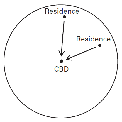

]

---

# Model assumptions
.pull-left[
* Recall the spatial equilibrium for workers, employers, and developers:
  - Income + Amenities - Housing Costs - Transportation Costs
  
*  **Holding income and amenities constant:**

- `\(\overline{Income} + \overline{Amenities}\)` **- (Housing Costs + Transportation Costs)**
  
  - These assumptions (income and amenities constant) imply that if transportation costs increase, housing costs must decrease in order to keep the utility constant over space
]

---
# Model assumptions

<br/>

* `\(x\)` is the distance from a consumer's residence to the CBD

* There is a cost associated with traveling `\(t\)` (e.g., gasoline, metro ticket)
  - Hence, the total commuting cost is `\(tx\)`. We apply the same `\(t\)` for everybody since they use the same transport mode

* One important implication is that **the disposable income `\(y-tx\)` decreases as `\(x\)` increases**

* Land is owned by absentee landlords (not in the city), builders rent land and build housing in a perfectly competitive market with CRS production

* Finally, the only difference between dwellings is their floor space

---
class: inverse,center, middle

# Consumer analysis

---

# Consumer analysis

* Consumers' problem: maximize their utility `\(U(q,c)\)` from consuming housing `\(q\)` and everything else `\(c\)` subject to their budget constraint `\(y - tx = pq + c\)`
  - `\(y - tx = pq + c\)`, where `\(p\)` is the price per square foot, and `\(q\)` is the floor space in a dwelling. Hence, rent is `\(pq\)`

* As stated before, the spatial equilibrium assumption (consumers equally well off everywhere in the city) together with the fact that amenities and income are held constant imply that there is a trade-off between transportation costs and housing costs
  - As distance increase from the CBD, commuting costs rise, and housing prices decline
  
--
  
* The lower `\(p\)` at distant suburban locations serves as a compensating differential

* You can think in "demand terms" - people want to live close to work, the demand for apartments near to the CBD will be higher, and the demand for apartments in the suburb will be lower

* Let's derive the inverse relationship between `\(p\)` and `\(x\)` using an indifference-curve diagram

---

# Consumer analysis
.pull-left[

* The suburban resident has a lower disposable income that the central-city consumer due to higher commuting costs

* Therefore, the price per square foot must fall, so the budget line allows the suburban consumer to reach the same indifference curve as her central-city counterpart

* Central-city resident consumes more food `\(c\)` than housing space. A suburban resident does the opposite, and dwelling size `\(q\)` rises as CBD's distance increases.

* To summarize, the model predicts `\(p \downarrow\)` as `\(x \uparrow\)` and `\(q \uparrow\)` as `\(x \uparrow\)`

]

# Consumer analysis
.pull-left[

* Two additional conclusions can be drawn from the consumer's analysis

* First, the price curve is convex. At a suburban location, dwellings are large, and a small decline in price per square foot generates enough housing-cost savings `\(pq\)` to compensate the extra mile of commute. At a central-city location, dwellings are small, and a large decrease in price is needed to generate the required savings.

* Second, the behavior of total rent `\(pq\)` is ambiguous

]

---

# Housing production analysis

---

# Housing production analysis
.pull-left[

* Now the focus shifts to the activities of housing developers. Then, we can see how the dwellings will look like in the model

* Builders' problem: maximize their profits. The revenue is `\(pQ\)`, where `\(Q=H(N,l)\)` is the floor space contained in a building as a function of land `\(l\)` and capital `\(N\)` (e.g., building materials).

* **The production function has a diminishing product of capital (N):** holding land fixed, the developers need extra doses of capital to increase the floor space. That means as the building gets taller, the developer needs to spend more and more in building materials (e.g., elevators)
]

# Housing production analysis
.pull-left[
* The production function has constant returns to scale. In other words, if the builder doubles both capital (N) and land (l), the building will have double floor space Q.

* As stated before, the developer will maximize profits by choosing capital and land for her building. **That decision also leads to a structure with a particular height**

* Revenues are equal to `\(pH(N,l)\)` and costs are equal to `\(rL+iN\)`. The developer leases the land from the owner for `\(r\)`, and the rental price of capital is `\(i\)` (exogenously determined).
]

# Housing production analysis
<br/>

* **The spatial equilibrium for developers implies that the profit from build apartments is the same everywhere**

* Since `\(p\)` decreases as `\(x\)` increases, the revenues from building distant from the CBD are lower. Hence, the land rental price must also fall as `\(x\)` increases, so the lower revenues are offset by lower costs.

* Again, the compensating differential can be viewed as demand-based. Developers compete vigorously for land in downtown because the revenues are higher there. This competition bids up land rents near to CBD. In the suburbs, lower demand leads to lower rent. In that way, the spatially uniform profit is achieved.

* The model thus predicts two other urban patterns. First, the land rent declines as CBD's distance increases. Then, this regularity generates the following pattern: **as land becomes more expensive compared to capital close to CBD**, developers will invest more in capital than in land in that area. That means they will build higher in downtown.

* Symbolically, `\(r \downarrow\)` as `\(x \uparrow\)`, building height `\(\downarrow\)` as `\(x \uparrow\)`

---

# Population density

* A final intracity regularity is the decline of population density (D) with distance to the CBD

* Since each dwelling contain one person, population density is just dwellings per `\(km^{2}\)`

* In the suburbs, people will consume more floor space in short buildings. Downtown has taller buildings with small dwellings. Hence, the population density is higher in the central city

* `\(D \downarrow\)` as `\(x \uparrow\)`

]

---

# Logical structure of the model
<br/>

---
class: inverse,center, middle

# Intercity Predictions

---
# The rural sector and the city's edge
.pull-left[

* Assume the city starts in equilibrium i.e., there is a balance between demand and supply of housing/the city fits its population

* The city's **land area** is a result of a competition between builders and farmers. We assume farmers are willing to pay `\(r_{A}\)` to rent productive land, which is independent of `\(x\)`. On the developer's side, `\(r\)` is convex just as `\(p\)` was (go back to slide 14)

* At the city's edge `\(\bar{x}\)`, the developers' bid rent curve `\(r\)` intersects the constant farmers' bid rent curve `\(r_{A}\)`.

* **The landowner rents the land to whoever pays more**
]

---
# A change in population

What happens when the total population increases?

.pull-left[1. Demand for housing will increase and will drive prices up everywhere in the city `\(p \uparrow\)`
2. With a higher price per square foot, people will consume less floor space `\(q \downarrow\)`
3. The higher `\(p\)` boosts builders profit, and they will again compete for land, driving land prices upward `\(r \uparrow\)`
4. The price of land `\(r\)` relative to the price of capital `\(i\)` is now higher, and developers will use more capital `\(N\)` relative to land: buildings are higher, apartments smaller. **Density increases everywhere**
5. The city fits more people pushing its edge, going back to equilibrium]

---
# A change in `\(r_{A}\)`

What happens when the agricultural rent is higher?

.pull-left[* `\(r_{A}\)` line goes up, and farmers now outbid developers for some areas inside of the city

* What about the people living there? Without that land (now occupied by farmers), the city does not fit its population. There will be an excess of demand for housing, and the process described earlier (when population size increases) repeats

* At the end, the city is spatially smaller, with taller buildings, smaller apartments, higher housing prices, and land rents, as well as higher population density
]

# A change in commuting costs

What happens when `\(t\)` increases?

.pull-left[* When the commuting cost increases, the former spatial equilibrium no longer holds - due to higher travel costs, suburban commuters can be better off moving closer to the center.

* Hence, the demand for downtown apartments is higher, bidding up their prices. On the other hand, the demand for suburban houses will decrease, driving those prices down.

* Same happens with land rents: due to higher profits in the center, developers will heavily compete for space there, driving up the land rent in the center. The opposite happens in the suburbs. **Therefore, the clockwise rotation**
]
.pull-right[![](figs/commute.png)]

---

# A change in commuting costs

**What happens in downtown?**
* Land is more expensive relative to capital. Hence, buildings are taller, apartments smaller.
* Central population density increases

**What happens in the suburb?**
* Land is cheaper relative to capital, and building heights fall in the city's suburbs
* What happens with floor space consumption `\(q\)` is ambiguous in the suburbs, as well as the change in population density

]