class: center, middle, inverse, title-slide # Econ 414 - Urban Economics ## Neighborhood Choice ### Marcelino Guerra ### April 15-20, 2021 --- # Introduction </br> * When a household chooses a house or an apartment, he or she is choosing much more than a dwelling * The AMM model describes a commuting-based residential choice * The hedonic model treats housing as a bundle of attributes * Voting with the feet model characterizes the consumer-voter's preference for local public goods provision * Now we shift the attention to neighborhood sorting - the consumers are also choosing neighbors who provide opportunities for social interactions within the community * We will see that in the U.S. cities, there is substantial segregation concerning income and educational attainment, as well as racial segregation * The goal of this lecture is to present empirical regularities within cities related to neighborhoods' socioeconomic composition. To explain the current patterns, we will use some social interaction models (tipping models). In the end, we discuss why integration matters --- class: inverse,center, middle # Educational Attainment and Income Segregation --- # Income Chicago-IL 2018 <iframe src="maps/income_chi.html" style="width: 1100px; height: 500px; border: 5px" alt=""> --- # Education Attainment Chicago-IL 2018 <iframe src="maps/educ_chi.html" style="width: 1100px; height: 500px; border: 5px" alt=""> --- class: inverse,center, middle # Neighborhood Choice --- # Competitive Bidding * Assume that positive externalities from neighbors increase with income, i.e., the willingness to pay for a particular neighborhood increases with the share of high-income households .pull-left[ * Consider a city with two neighborhoods: A and B. Each community has 100 households, and each resident occupies one unit of land. Half of the city's population is high-income and half low-income * The Figure shows the difference in land rent between neighborhoods A and B as the share of high-income households changes * At point `\(i\)`, neighborhoods A and B have 50 households from each income level * Equilibrium requires that all households in a particular neighborhood pay the same rent ] .pull-right[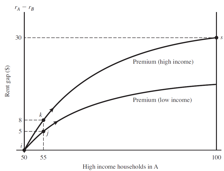] --- # Competitive Bidding: Segregation * Suppose neighborhood A is split into 55 households in the high-income group and 45 in the low-income group. That means neighborhood B has the opposite distribution 45 high-income consumers and 55 low-income neighbors .pull-left[ * At this point, high-income households are willing to pay an $8 premium for living in neighborhood A. That is higher than the low-income household's willingness to pay * High-income households in neighborhood B will outbid low-income residents in A. That will move the equilibrium far away from `\(i\)` and up to `\(s\)` * In the end, the two neighborhoods will be entirely segregated by income ] .pull-right[] --- # Competitive Bidding: Integration * In the previous example, integration was an unstable equilibrium: any small increase in the share of high-income residents in A would lead to complete segregation .pull-left[ * Now, consider the case where low-income households have a steeper premium curve - they always outbid wealthy residents * The number of low-income households will increase at the expense of high-income residents * If the composition of the neighborhoods start at any point other than `\(i\)`, low-income residents will outbid high-income residents, and there will be complete integration at the end ] .pull-right[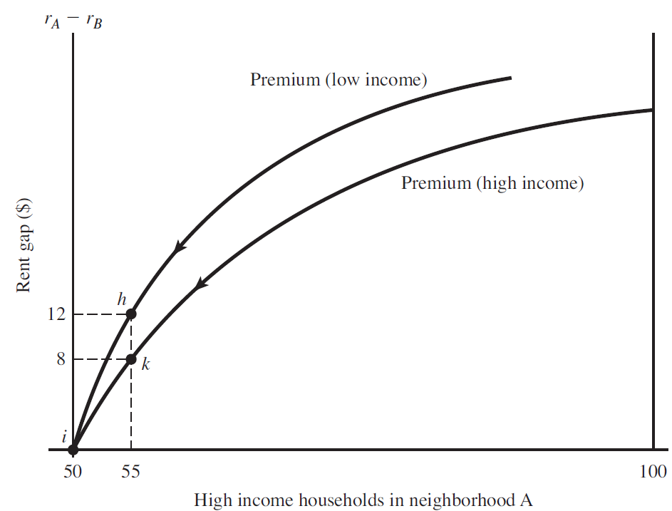] --- # Competitive Bidding: Mix * A third possibility is something in between total integration and completely segregation. In this case, the two premium curves for neighborhood A intersects at 70%. The composition of area A is 70 high income and 30 low-income residents. In neighborhood B, the arrangement is the opposite (30/70) .pull-left[ * `\(m\)` **is a stable equilibrium**. Suppose there are 75 high-income residents in A. The low-income residents in B would outbid high-income households in A - `\(g>f\)` -, bringing the share of wealthy residents back to 70%. * The same reasoning can be applied to points `\(d\)` and `\(e\)`. When there are only 65 wealthy residents in neighborhood A, high-income households in B will outbid low-income households in A, bringing back the 70/30 equilibrium ] .pull-right[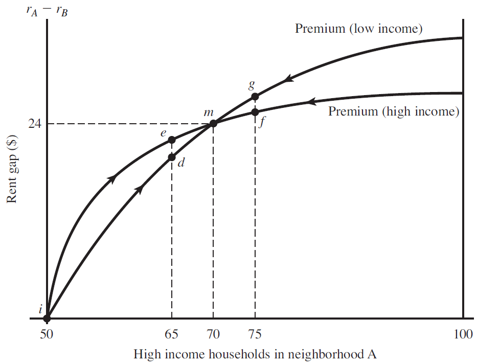] --- # Lot Size, Fiscal Zoning and Segregation * In the competitive bidding model, we assume that each household occupies one unit of land. However, land consumption can increase with income. .pull-left[ * Consider the former case of total segregation. A wealthy resident is willing to pay an $8 premium to live with 55 high-income households while a low-income resident is willing to pay only 5. If the wealthy resident consumes more land - let's say two units -, then the high-income premium is 4 dollars per unit of land. That is less than 5 dollars - the premium that low-income households are willing to pay * Now, the low-income households outbid the wealthy residents when the share of high-income households is higher than 50. In this case, in any deviation from 50/50, the low-income families will outbid the wealthy residents, and there will be integration in equilibrium ] .pull-right[] --- # Lot Size, Fiscal Zoning and Segregation * We just saw one implication of variable lot sizes for neighborhood choice: when high-income residents consume more land, integration is more likely .pull-left[ * Some local governments use minimum lot size zoning to regulate land use * One of the consequences of this policy is segregation * Consider the former example again. If the government requires a minimum lot size of two units, the wealthy residents in B will outbid low-income households in A - a $4 premium per unit land versus 2.5 dollars - for any share of high-income households in A greater than 50% * At the end, the two neighborhoods will be completely segregated by income ] .pull-right[] --- # Tipping point </br> * One of the key features of social interaction models is that preferences depend on other agent's choices. We just saw that households were willing to pay a premium for living in a neighborhood with a higher share of wealthy residents * In the first example, **an integrated neighborhood** (50 low income/50 high income) **was an unstable equilibrium**. When the share of wealthy residents was a little bit more than 50%, suddenly the neighborhood turned towards 100% high-income households * Another way to think about this is the following: even if residents have mild preferences for neighbors like them, that could drive the neighborhood to entire segregation. Check the **[parable of the polygons](https://ncase.me/polygons/)** * This idea can be used to explore neighborhood tipping. Tipping occurs when a new minority group enters a neighborhood, and that causes the earlier residents to begin evacuating --- # Some Empirical Evidence of Tipping * [Card, Mas and Rothstein (2008)](https://davidcard.berkeley.edu/papers/tipping-dynamics.pdf) provide evidence that white population flows exhibit tipping-like behavior in most U.S. cities. They use Census tract data from 1970 through 2000 .pull-left[ * The tipping points rage from 5% to 20% minority share * The figure shows the example of Chicago. The y-axis is the mean percentage changes in the Chicago Census tracts' white population from 1970 to 1980. The x-axis is the minority share (nonwhites and white Hispanics) in 1970 * One can see a discontinuity in the plot. There are white population gains when the share of the minority is less than 5% (vertical line). Also, there are substantial outflows when the share of the minority is higher than 5%. That is, 5% minority share is the tipping point in Chicago neighborhoods during 1970-1980 * The discontinuity is less well defined for 1990-2000 ] .pull-right[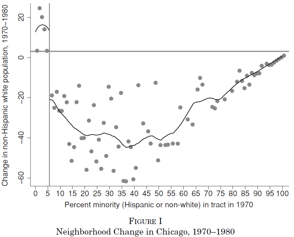] --- class: inverse,center, middle # Racial Segregation --- # Racial Composition Chicago-IL 2018 <iframe src="maps/black_chi.html" style="width: 1100px; height: 500px; border: 5px" alt=""> --- # Segregation in U.S. counties 2018 <iframe src="maps/RDI.html" style="width: 1100px; height: 500px; border: 5px" alt=""> --- # Theories of Segregation </br> 1. Self-segregation * Ghettos are a mechanism to help a group assimilate into a new environment, and members of minorities have a stronger taste for living among members of the same ethnic group 2. Collective Action Racism * Ghettos are a result of collective actions taken by the majority group to enforce separation from the minority. Examples: legal barriers to minority mobility such as racial zoning and redlining mortgage on a racial basis, and explicit/implicit threats of violence that discourage minorities from moving into white neighborhoods 3. White Flight * Segregation is enforced by individual whites' decisions to live among themselves - whites are willing to pay more than blacks to live in predominantly white neighborhoods --- # Explaining Segregation </br> * [Cutler, Glaeser and Vigdor (1999)](https://dash.harvard.edu/bitstream/handle/1/2770033/Cutler_RiseandFall.pdf) differentiate the segregation theories looking at housing costs for blacks and whites. Assume the competitive bidding setting we saw before but replace high-income/low-income by blacks and whites * If increases in white flight cause increases in segregation, whites will pay relatively more for housing than blacks as segregation rises. Alternatively, if increases in segregation are caused by increases in collective action racism or by self-segregation, blacks will pay relatively more for housing than whites in more segregated cities * The authors further differentiate self-segregation from collective action racism by looking at housing prices for different black populations. Self-segregation is more likely for new black migrants compared to long-term black residents. In the case of collective action racism, all blacks would pay a higher premium in more segregated cities * Cutler, Glaeser and Vigdor (1999) findings point to * For 1940 and 1970, segregation can be explained by collective actions on the part of whites to exclude blacks * By 1990, it appears that differences in residential location between blacks and whites occur due to white flight --- # Consequences of Segregation </br> * Neighborhood effects * The concentration of low-income households generates harmful spillovers. Neighborhoods with a high unemployment rate have less information about job openings. * Increase in segregation increases the probability of dropping out of high school. Segregation also leads to lower employment rates and higher rates of single parenthood * Black residents in segregated areas earn less, and segregation raises the black poverty rate * Spatial Mismatch * Location matters in the urban labor market. A segment of the workforce that is concentrated in an area far from jobs will have a relatively low employment rate * Devaluation of Financial Assets * [Houses in majority-black neighborhoods sell at a 20 percent or more significant discount to otherwise similar homes in predominantly white areas](https://cityobservatory.org/the-devaluation-of-black-neighborhoods-part-1/) --- # Segregation Trends in the U.S. .pull-left[ * The figure reports the average segregation experienced by the typical urban black resident from 1890 to 2010 * Between 1910 and 1960, blacks moved to urban areas in vast numbers. They often faced legal obstacles in their choice of neighborhood - collective action racism. As a consequence, segregation rose * As of 2010, the dissimilarity index had declined to its lowest level in a century * Between 2000 and 2010, segregation declined in all the ten largest metro areas * Currently, Chicago's dissimilarity index is around 72. In 1970, that value topped 90 percent ] .pull-right[ **Source:** Glaeser and Vigdor (2012)] --- # Why has segregation declined? <br/> * The successful fight for housing freedom that culminated with the 1968 Fair Housing Act * Significant shifts in public attitudes toward integration * American neighborhoods with no black residents has decreased by more than 90% over the past 50 years * Depopulation of ghettos * African-American suburbanization * Interregional Migration. Blacks moving from North/Midwest to the Sun Belt region * The demolition of segregated high-rise housing projects since 1970 * Gentrification and immigration have made a dent in segregation